")


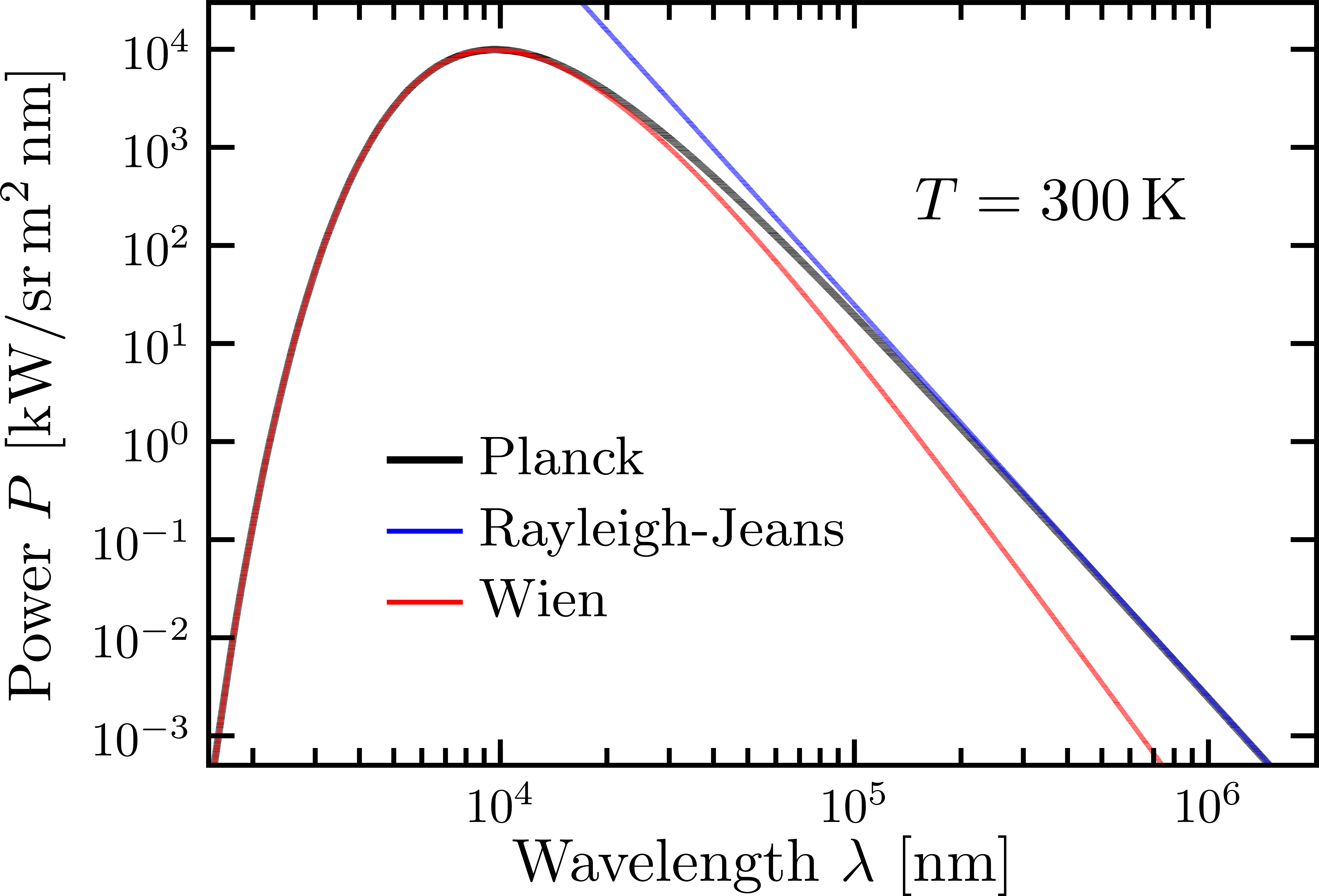
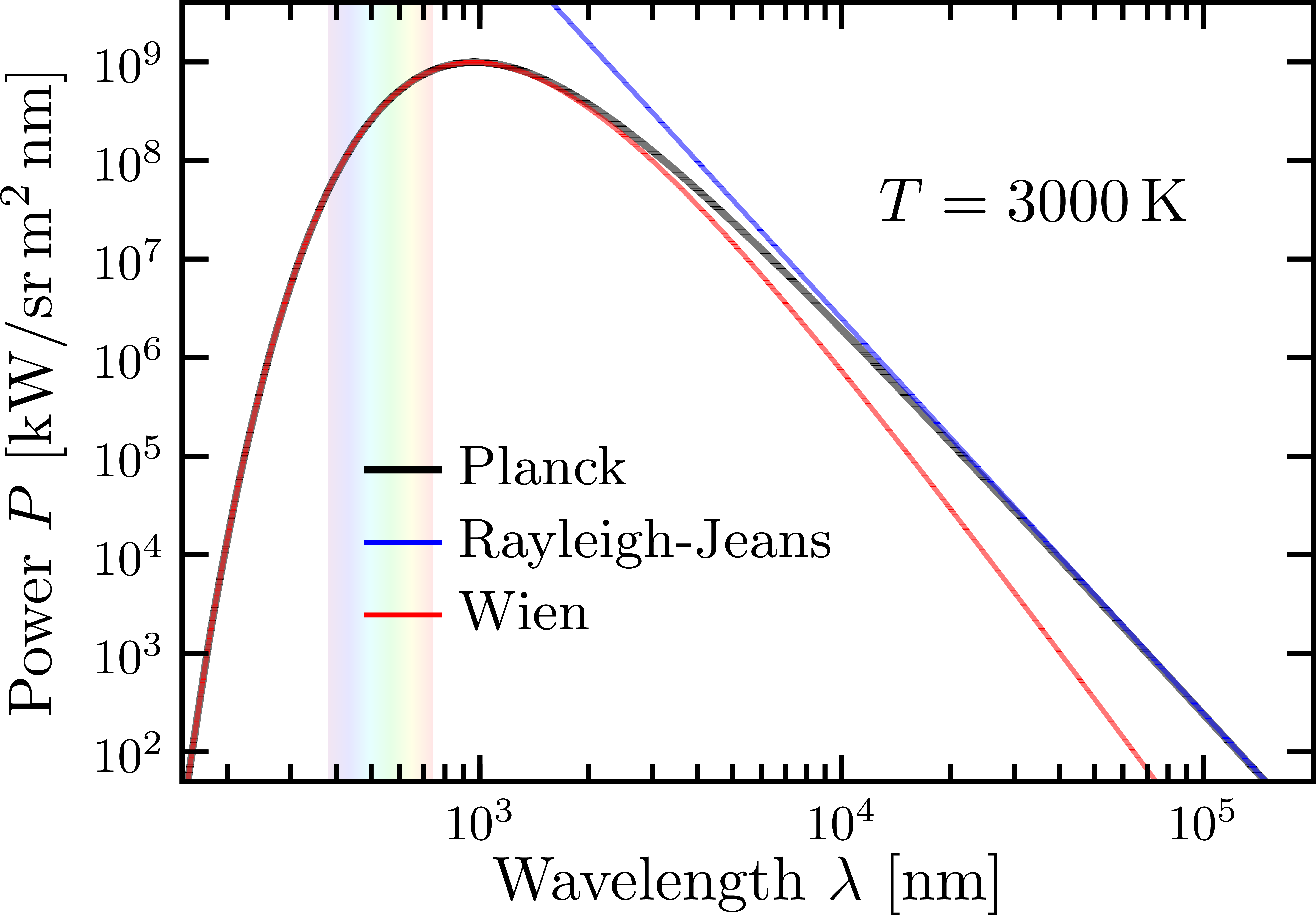
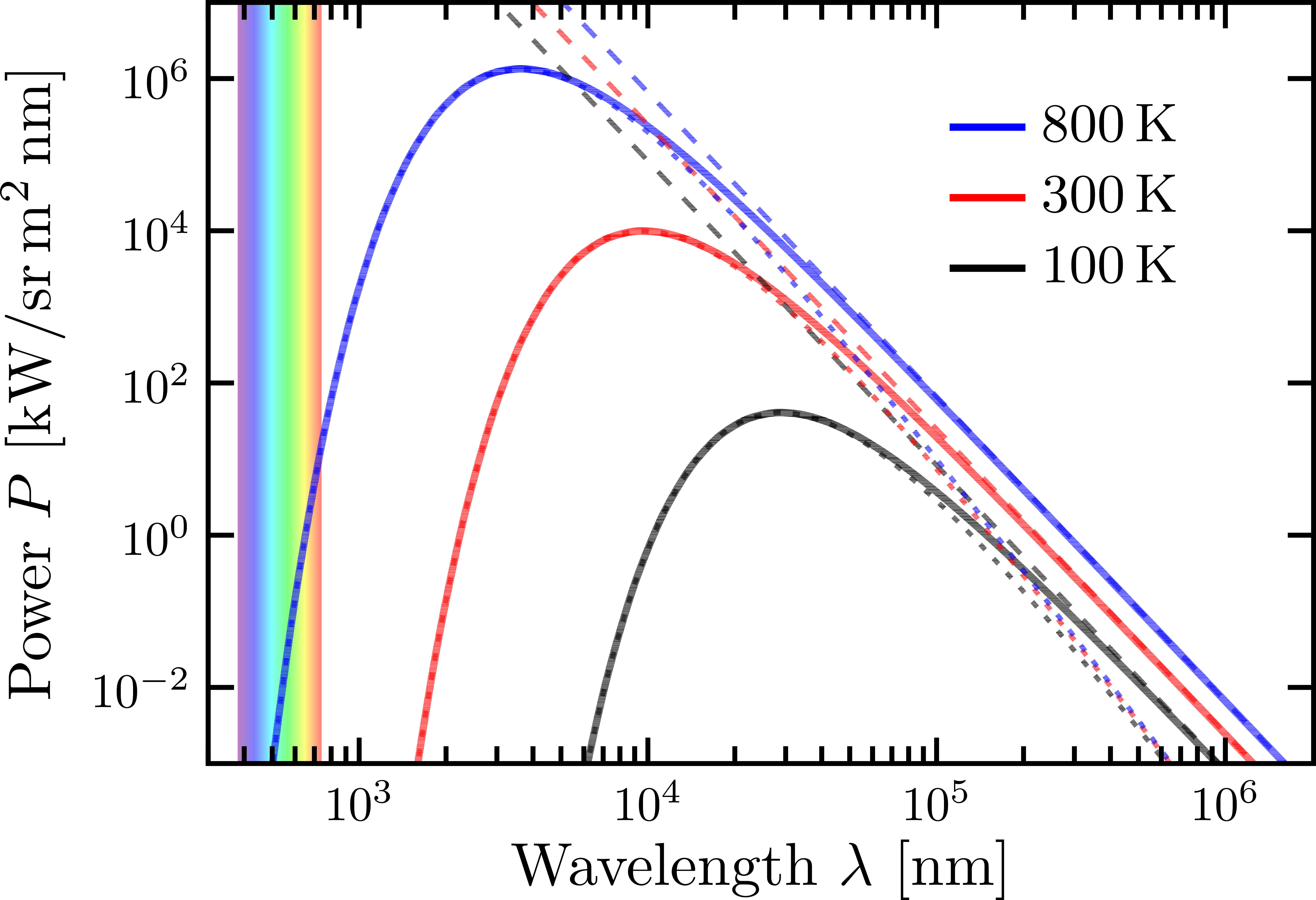
Plot of black body formulas: Rayleigh-Jeans, Wien and Planck. Inspiration from Wikipedia.
Find other black body diagrams via the “black body” tag: black body color gradient, cavity model, Plank oscillators. For more figures related to thermodynamics, see the “thermodynamics” category.
Including Wien's displacement law:
Comparing black body colors in a log-log plot:
Comparing Planck to Rayleigh-Jeans & Wien in a log-log plot for T = 300 K:
For T = 3000 K:
Comparison for several temperatures:
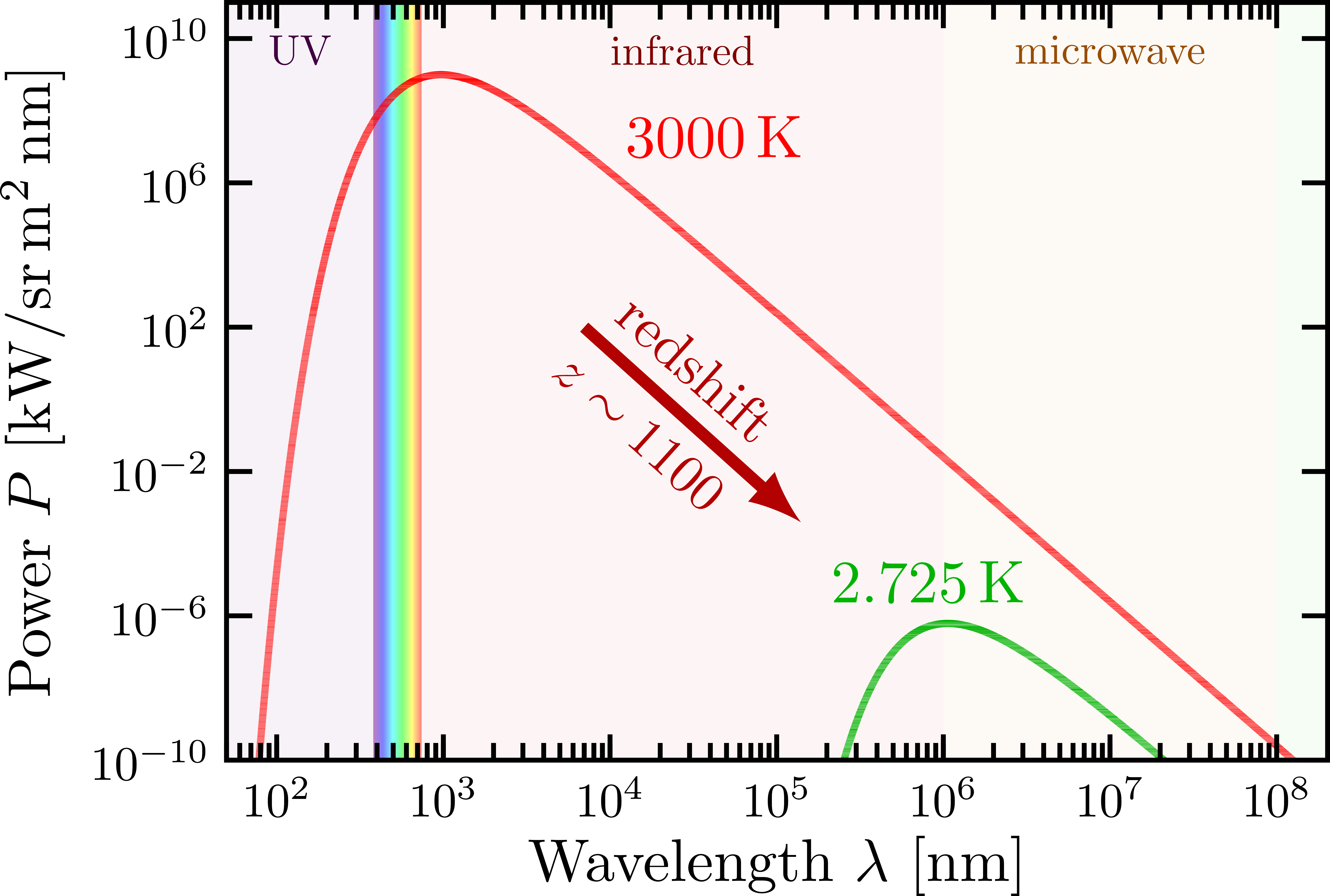
Redshift of the cosmic microwave background (CMB) from 3000K to ~3K due to the expansion of the universe:
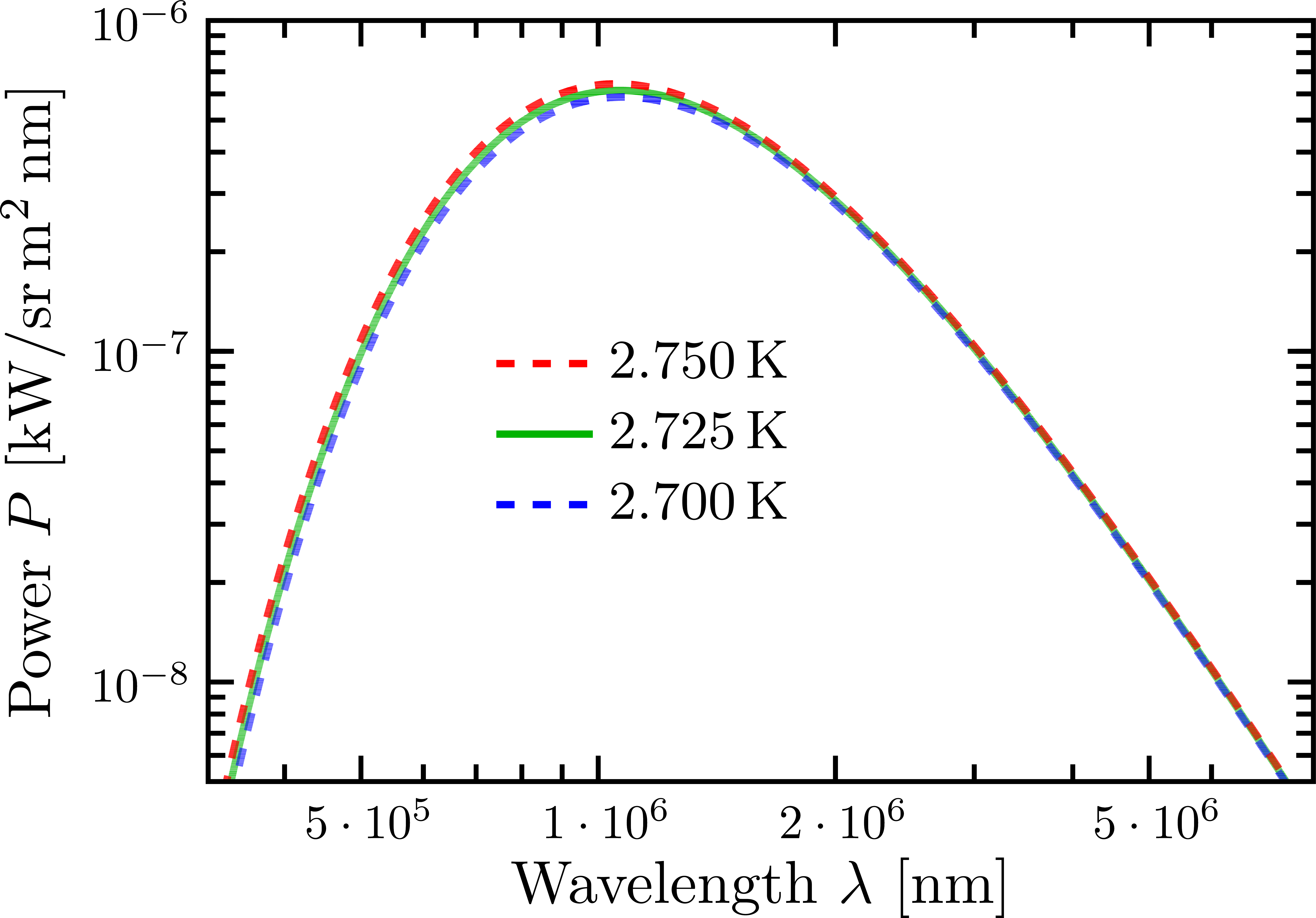
Small variations of the CMB temperature (note real variation are actually on the order of ΔT ~ 20 𝜇K after subtracting the dipole ΔT ~ 3 mK due to the Doppler effect of our motion relative to the CMB):
Edit and compile if you like:
% Author: Izaak Neutelings (March 2019)
\documentclass[border=3pt,tikz]{standalone}
\tikzset{>=latex} % for LaTeX arrow head
\usepackage{pgfplots} % for the axis environment
\pgfplotsset{
  compat=1.13, % TikZ coordinates <-> axes coordinates
  /pgf/number format/1000 sep={},
  legend image code/.code={
    \draw[mark repeat=2,mark phase=2]
    plot coordinates {(0cm,0cm) (0.22cm,0cm) (0.44cm,0cm)};%
  }
}
\usepackage{siunitx}

% redraw axis on top
\makeatletter \newcommand{\pgfplotsdrawaxis}{\pgfplots@draw@axis} \makeatother
\pgfplotsset{axis line on top/.style={after end axis/.append code={\pgfplotsdrawaxis}}
}

% CUSTOM COLORS
% See https://tikz.net/blackbody_color/
\definecolor{1000K}{rgb}{1,0.0337,0}
\definecolor{2000K}{rgb}{1,0.2647,0.0033}
\definecolor{3000K}{rgb}{1,0.4870,0.1411}
\definecolor{4000K}{rgb}{1,0.6636,0.3583}
\definecolor{5000K}{rgb}{1,0.7992,0.6045}
\definecolor{6000K}{rgb}{1,0.9019,0.8473}
\definecolor{8000K}{rgb}{0.7874,0.8187,1}
\definecolor{10000K}{rgb}{0.6268,0.7039,1}
\pgfdeclareverticalshading{rainbow}{100bp}{
  color(0bp)=(red); color(25bp)=(red); color(35bp)=(yellow);
  color(45bp)=(green); color(55bp)=(cyan); color(65bp)=(blue);
  color(75bp)=(violet); color(100bp)=(violet)
}
\colorlet{myred}{red!70!black}
\colorlet{mygreen}{green!70!black}
\colorlet{mydarkgreen}{green!55!black}

% PLANCK & RAYLEIGH-JEANS
% 2hc^2/lambda^5 = 2 * 6.62607015e-34 * 299792458^2
%                = 1.191042972e-16
%    W.m -> kW.nm: 1.191042972e26
%  hc/k lambda T = 6.62607015e-34*299792458/(1.38064852e-23)
%                = 0.01438777378
%         m -> nm: 0.01438777378e9
% 2ckT/lambda^4  = 2 * 299792458 * 1.38064852e-23
%                = 8.278160269e-15
%    W.m -> kW.nm: 8.278160269e18
\pgfmathdeclarefunction{planck}{2}{%
  \pgfmathparse{1.191042972e26/(#1^5)/(exp(0.01439e9/(#1*#2))-1)}%
}
\pgfmathdeclarefunction{rayleighjeans}{2}{%
  \pgfmathparse{8.278160269e18*#2/(#1^4)}%
}
\pgfmathdeclarefunction{wien}{2}{%
  \pgfmathparse{1.191042972e26/(#1^5)*exp(-0.01439e9/(#1*#2))}%
}
\pgfmathdeclarefunction{lampeak}{1}{% % Wien's displacement law
  \pgfmathparse{2.898e6/#1}%
}

\begin{document}


% BLACK BODY - 3000, 4000, 5000K
\begin{tikzpicture}
  \message{^^JBlack body}
  \def\N{60}
  \def\xmax{3100}
  \def\ymax{1.36e10}
  \def\tick#1#2{\draw[thick] (#1+.01*\ymax) -- (#1-.01*\ymax) node[below=-.5pt,scale=0.75] {#2};}
  \begin{axis}[
      every axis plot/.style={
        mark=none,samples=\N,domain=5:\xmax,smooth},
      xmin=(-.05*\xmax), xmax=(1.05*\xmax),
      ymin=(-.08*\ymax), ymax=(1.08*\ymax),
      restrict y to domain=0:\ymax,
      axis lines=middle,
      axis line style=thick,
      %enlargelimits=upper, % extend the axes a bit to the right and top
      tick style={black,thick},
      ticklabel style={scale=0.8},
      %xtick style={draw=none},xticklabels=none,
      max space between ticks=26,
      xlabel={Wavelength $\lambda$ [nm]},
      ylabel={Power $P$ [kW/sr\,m$^2$\,nm]},
      xlabel style={at={(rel axis cs:0.5,0)},below=-1pt,font=\small},
      ylabel style={at={(rel axis cs:-0.11,0.5)},rotate=90},
      width=9cm, height=7cm,
      %clip=false
      tick scale binop=\times,
      every y tick scale label/.style={at={(rel axis cs:0,1)},anchor=south}]
    ]

    % RAINBOW
    \shade[shading=rainbow,shading angle=90,opacity=0.5] (380,0) rectangle (740,\ymax);
    \node[above=-1pt,scale=0.8] at (200,\ymax) {\strut UV}; % 10 - 400 nm
    \node[above=-1pt,scale=0.8] at (570,\ymax) {\strut optical}; % 380 - 740 nm
    \node[above=-1pt,scale=0.8] at (920,\ymax) {\strut IR}; % 740 - 1050 nm

    % PLANCK
    \addplot[very thick,red]    {planck(x,3000)};
    \addplot[very thick,orange] {planck(x,4000)};
    \addplot[very thick,samples=3*\N,blue] {planck(x,5000)};
    %\addplot[dashed,thick,red,domain=1000:4000]    {rayleighjeans(x,3000)};
    %\addplot[dashed,thick,orange,domain=1000:4000] {rayleighjeans(x,4000)};
    \addplot[dashed,thick,blue,domain=1000:4000]   {rayleighjeans(x,5000)};
    %\addplot[dashed,thick,red,domain=1000:4000]    {wien(x,3000)};
    %\addplot[dashed,thick,orange,domain=1000:4000] {wien(x,4000)};
    %\addplot[dashed,thick,blue,domain=1000:4000]   {wien(x,5000)};

    %% MAXIMUM (Wien's displacement law)
    %\addplot[mygreen,very thin,variable=T,domain=2500:6000]
    %  ({lampeak(T)},{planck(lampeak(T),T)});

    % LABELS
    \node[above=0pt,scale=0.75,red] at (1150,{planck(1150,3000)}) {\SI{3000}{K}};
    \node[above right=-1pt,scale=0.75,orange!80!black] at (740,{planck(740,4000)}) {\SI{4000}{K}};
    \node[above right=-1pt,scale=0.75,blue] at (800,{planck(800,5000)}) {\SI{5000}{K}};
    \node[above right=-1pt,scale=0.75,blue] at (1500,{rayleighjeans(1500,5000)}) {\SI{5000}{K} Rayleigh-Jeans};

    %% TICKS
    %\tick{500,0}{500}
    %\tick{1000,0}{1000}
    %\tick{1500,0}{1500}
    %\tick{2000,0}{2000}
    %\tick{2500,0}{2500}
    %\tick{3000,0}{3000}

  \end{axis}
\end{tikzpicture}


% BLACK BODY - 3000, 4000, 5000K, Wien's displacement law
\begin{tikzpicture}
  \message{^^JBlack body, Wien's displacement law}
  \def\N{60}
  \def\xmax{3100}
  \def\ymax{1.36e10}
  \def\tick#1#2{\draw[thick] (#1+.01*\ymax) -- (#1-.01*\ymax) node[below=-.5pt,scale=0.75] {#2};}
  \begin{axis}[
      every axis plot/.style={
        very thick,mark=none,samples=\N,domain=5:\xmax,smooth},
      xmin=(-.05*\xmax), xmax=(1.05*\xmax),
      ymin=(-.08*\ymax), ymax=(1.08*\ymax),
      restrict y to domain=0:\ymax,
      axis lines=middle,
      axis line style=thick,
      %enlargelimits=upper, % extend the axes a bit to the right and top
      tick style={black,thick},
      ticklabel style={scale=0.8},
      %xtick style={draw=none},xticklabels=none,
      max space between ticks=26,
      xlabel={Wavelength $\lambda$ [nm]},
      ylabel={Power $P$ [kW/sr\,m$^2$\,nm]},
      xlabel style={at={(rel axis cs:0.5,0)},below=-1pt,font=\small},
      ylabel style={at={(rel axis cs:-0.11,0.5)},rotate=90},
      width=9cm, height=7cm,
      %clip=false
      tick scale binop=\times,
      every y tick scale label/.style={at={(rel axis cs:0,1)},anchor=south}]
    ]

    % RAINBOW
    \shade[shading=rainbow,shading angle=90,opacity=0.5] (380,0) rectangle (740,\ymax);
    \node[above=-1pt,scale=0.8] at (200,\ymax) {\strut UV}; % 10 - 400 nm
    \node[above=-1pt,scale=0.8] at (570,\ymax) {\strut optical}; % 380 - 740 nm
    \node[above=-1pt,scale=0.8] at (920,\ymax) {\strut IR}; % 740 - 1050 nm

    % PLANCK
    \addplot[red]    {planck(x,3000)};
    \addplot[orange] {planck(x,4000)};
    \addplot[blue,samples=3*\N] {planck(x,5000)};
    \addplot[dashed,thick,blue,domain=1000:3500] {rayleighjeans(x,5000)};

    % MAXIMUM (Wien's displacement law)
    \addplot[mydarkgreen,thick,variable=T,domain=2200:4000,samples=40]
      ({lampeak(T)},{planck(lampeak(T),T)});
    \addplot[mydarkgreen,thick,variable=T,domain=4000:5200,samples=100]
      ({lampeak(T)},{planck(lampeak(T),T)});
    \fill[mydarkgreen!80!black] ({lampeak(3000)},{planck(lampeak(3000),3000)}) circle(1.5pt);
    \fill[mydarkgreen!80!black] ({lampeak(4000)},{planck(lampeak(4000),4000)}) circle(1.5pt);
    \fill[mydarkgreen!80!black] ({lampeak(5000)},{planck(lampeak(5000),5000)}) circle(1.5pt);

    % LABELS
    \node[above=0pt,scale=0.75,red] at (1150,{planck(1150,3000)}) {\SI{3000}{K}};
    \node[above right=-1pt,scale=0.75,orange!80!black] at (740,{planck(740,4000)}) {\SI{4000}{K}};
    \node[above right=-1pt,scale=0.75,blue] at (800,{planck(800,5000)}) {\SI{5000}{K}};
    \node[above right=-1pt,scale=0.75,blue] at (1500,{rayleighjeans(1500,5000)}) {\SI{5000}{K} Rayleigh-Jeans};

  \end{axis}
\end{tikzpicture}


% BLACK BODY - 3000, 4000, 5000K
\begin{tikzpicture}
  \message{^^JBlack body}
  \def\N{60}
  \def\xmax{3100}
  \def\ymax{1.43e10}
  \def\tick#1#2{\draw[thick] (#1+.01*\ymax) -- (#1-.01*\ymax) node[below=-.5pt,scale=0.75] {#2};}
  \begin{axis}[
      every axis plot/.style={
        mark=none,samples=\N,domain=5:\xmax,smooth},
      xmin=(0), xmax=(\xmax),
      ymin=(0), ymax=(\ymax),
      restrict y to domain=0:\ymax,
      %axis lines=middle,
      axis line style=thick,
      tick style={black,thick},
      ticklabel style={scale=0.8},
      xlabel={Wavelength $\lambda$ [nm]},
      ylabel={Power $P$ [kW/sr\,m$^2$\,nm]},
      xlabel style={below=-1pt,font=\small},
      ylabel style={above=-1pt},
      width=9cm, height=7cm,
      tick scale binop=\times,
      every y tick scale label/.style={at={(rel axis cs:0,1)},anchor=south}]
    ]

    % RAINBOW
    \draw[dashed] (380,{planck(380,5000)}) -- (380,\ymax);
    \draw[dashed] (740,{planck(740,5000)}) -- (740,\ymax);
    \begin{scope}
      \clip[variable=\x,domain=200:1000,samples=40]
        plot(\x,{planck(\x,5000)}) |- (200,0) -- cycle;
      \shade[shading=rainbow,shading angle=90,opacity=0.7] (380,0) rectangle (740,\ymax);
    \end{scope}

    % PLANCK
    \addplot[very thick,red]    {planck(x,3000)};
    \addplot[very thick,orange] {planck(x,4000)};
    \addplot[very thick,samples=3*\N,blue] {planck(x,5000)};
    \addplot[dashed,thick,blue,domain=1000:4000]   {rayleighjeans(x,5000)};

    % MAXIMUM (Wien's displacement law)
    \addplot[mydarkgreen,thick,variable=T,domain=2200:4000,samples=40]
      ({lampeak(T)},{planck(lampeak(T),T)});
    \addplot[mydarkgreen,thick,variable=T,domain=4000:5000,samples=100]
      ({lampeak(T)},{planck(lampeak(T),T)});
    \fill[mydarkgreen!80!black] ({lampeak(3000)},{planck(lampeak(3000),3000)}) circle(1.5pt);
    \fill[mydarkgreen!80!black] ({lampeak(4000)},{planck(lampeak(4000),4000)}) circle(1.5pt);
    \fill[mydarkgreen!80!black] ({lampeak(5000)},{planck(lampeak(5000),5000)}) circle(1.5pt);

    % LABELS
    \node[above=0pt,scale=0.75,red]
      at (1150,{planck(1150,3000)}) {\SI{3000}{K}};
    \node[above right=-1pt,scale=0.75,orange!80!black]
      at (740,{planck(740,4000)}) {\SI{4000}{K}};
    \node[above right=-1pt,scale=0.75,blue]
      at (800,{planck(800,5000)}) {\SI{5000}{K}};
    \node[above right=-1pt,scale=0.75,blue]
      at (1500,{rayleighjeans(1500,5000)}) {\SI{5000}{K} Rayleigh-Jeans};

    % LABELS
    \node[below=2pt,scale=0.8] at (200,\ymax) {\strut UV}; % 10 - 400 nm
    \node[below=2pt,scale=0.8] at (562,\ymax) {\strut optical}; % 380 - 740 nm
    \node[below=2pt,scale=0.8] at (920,\ymax) {\strut IR}; % 740 - 1050 nm

  \end{axis}
\end{tikzpicture}


% BLACK BODY LOG-LOG - colors
% See https://tikz.net/blackbody_color/
\begin{tikzpicture} %[scale=2]
  \message{^^JBlack body colors}
  \def\N{40}
  \def\xmin{35}
  \def\xmax{1.7e5}
  \def\ymin{1e2}
  \def\ymax{2e12}
  \begin{loglogaxis}[
      every axis plot post/.append style={
        very thick,mark=none,domain=\xmin:\xmax,samples=\N,smooth},
      xmin=\xmin, xmax=(1.01*\xmax),
      ymin=\ymin, ymax=\ymax,
      restrict y to domain=0.1*\ymin:\ymax,
      log basis y=10,
      axis line style=thick,
      tick style={black,thick},
      ticklabel style={scale=0.8},
      max space between ticks=23,
      yminorticks=false,
      xlabel={Wavelength $\lambda$ [nm]},
      ylabel={Power $P$ [kW/sr\,m$^2$\,nm]},
      xlabel style={at={(rel axis cs:0.5,0)},below=8pt},
      ylabel style={above=-2pt},
      legend style={at={(0.98,0.95)},anchor=north east,draw=none,fill=none,
                    nodes={scale=0.7, transform shape}},
      legend cell align={left},
      width=8cm, height=6cm,
      axis line on top
    ]

    % RAINBOW
    \shade[shading=rainbow,shading angle=90,opacity=0.5] (380,\ymin) rectangle (740,\ymax);

    % PLANCK
    \addplot[10000K] {planck(x,10000)};
    \addplot[6000K]  {planck(x,7500)};
    \addplot[5000K]  {planck(x,5000)};
    \addplot[3000K]  {planck(x,3000)};
    \addplot[2000K]  {planck(x,2000)};
    \addplot[1000K]  {planck(x,1000)};
    \addplot[black]  {planck(x, 500)};
    %\addplot[dashed,thick,black] {rayleighjeans(x,500)};

    % LEGENDS
    \addlegendentry{\SI{10000}{K}}
    \addlegendentry{\SI{7500}{K}}
    \addlegendentry{\SI{5000}{K}}
    \addlegendentry{\SI{3000}{K}}
    \addlegendentry{\SI{2000}{K}}
    \addlegendentry{\SI{1000}{K}}
    \addlegendentry{\SI{500}{K}}

  \end{loglogaxis}
\end{tikzpicture}


% BLACK BODY LOG-LOG - Rayleigh-Jeans / Wien, 300K
\begin{tikzpicture}
  \message{^^JRayleigh-Jeans / Wien, 300K}
  \def\N{40}
  \def\xmin{1.5e3}
  \def\xmax{2e6}
  \def\ymin{5e-4}
  \def\ymax{3e4}
  \begin{loglogaxis}[
      every axis plot/.style={
        very thick,mark=none,domain=\xmin:\xmax,samples=\N,smooth},
      xmin=\xmin, xmax=(1.01*\xmax),
      ymin=\ymin, ymax=\ymax,
      restrict y to domain=0.1*\ymin:\ymax,
      log basis y=10,
      axis line style=thick,
      tick style={black,thick},
      ticklabel style={scale=0.8},
      %ticks=none,
      max space between ticks=23,
      yminorticks=false,
      xlabel={Wavelength $\lambda$ [nm]},
      ylabel={Power $P$ [kW/sr\,m$^2$\,nm]},
      xlabel style={at={(rel axis cs:0.5,0)},below=8pt},
      ylabel style={above=-2pt},
      width=8cm, height=6cm,
      legend style={at={(0.14,0.15)},anchor=south west,draw=none,fill=none,font=\small},
      legend cell align={left},
      axis line on top
    ]

    % PLANCK
    \addplot[black]      {planck(x,300)};
    \addplot[thick,blue] {rayleighjeans(x,300)};
    \addplot[thick,red]  {wien(x,300)};

    % LEGENDS
    \addlegendentry{Planck}
    \addlegendentry{Rayleigh-Jeans}
    \addlegendentry{Wien}
    \node[scale=1] at (0.18*\xmax,0.01*\ymax) {$T=\SI{300}{K}$};

  \end{loglogaxis}
\end{tikzpicture}


% BLACK BODY LOG-LOG - Rayleigh-Jeans / Wien, 3000K
\begin{tikzpicture}
  \message{^^JRayleigh-Jeans / Wien, 3000K}
  \def\N{40}
  \def\xmin{1.5e2}
  \def\xmax{2e5}
  \def\ymin{5e1}
  \def\ymax{4e9}
  \begin{loglogaxis}[
      every axis plot/.style={
        very thick,mark=none,domain=\xmin:\xmax,samples=\N,smooth},
      xmin=\xmin, xmax=(1.01*\xmax),
      ymin=\ymin, ymax=\ymax,
      restrict y to domain=0.1*\ymin:\ymax,
      log basis y=10,
      axis line style=thick,
      tick style={black,thick},
      ticklabel style={scale=0.8},
      %ticks=none,
      max space between ticks=23,
      yminorticks=false,
      xlabel={Wavelength $\lambda$ [nm]},
      ylabel={Power $P$ [kW/sr\,m$^2$\,nm]},
      xlabel style={at={(rel axis cs:0.5,0)},below=8pt},
      ylabel style={above=-2pt},
      width=8cm, height=6cm,
      legend style={at={(0.14,0.15)},anchor=south west,draw=none,fill=none,font=\small},
      legend cell align={left},
      axis line on top
    ]

    % RAINBOW
    \shade[shading=rainbow,shading angle=90,opacity=0.1] (380,\ymin) rectangle (740,\ymax);

    % PLANCK
    \addplot[black]      {planck(x,3000)};
    \addplot[thick,blue] {rayleighjeans(x,3000)};
    \addplot[thick,red]  {wien(x,3000)};

    % LEGENDS
    \addlegendentry{Planck}
    \addlegendentry{Rayleigh-Jeans}
    \addlegendentry{Wien}
    \node[scale=1] at (0.17*\xmax,0.01*\ymax) {$T=\SI{3000}{K}$};

  \end{loglogaxis}
\end{tikzpicture}


% BLACK BODY LOG-LOG - Rayleigh-Jeans / Wien
\begin{tikzpicture}
  \message{^^JRayleigh-Jeans / Wien}
  \def\N{40}
  \def\xmin{3e2}
  \def\xmax{2e6}
  \def\ymin{1e-3}
  \def\ymax{1e7}
  \begin{loglogaxis}[
      every axis plot/.style={
        very thick,mark=none,domain=\xmin:\xmax,samples=\N,smooth},
      xmin=\xmin, xmax=(1.01*\xmax),
      ymin=\ymin, ymax=\ymax,
      restrict y to domain=0.1*\ymin:\ymax,
      log basis y=10,
      axis line style=thick,
      tick style={black,thick},
      ticklabel style={scale=0.8},
      %ticks=none,
      max space between ticks=23,
      yminorticks=false,
      xlabel={Wavelength $\lambda$ [nm]},
      ylabel={Power $P$ [kW/sr\,m$^2$\,nm]},
      xlabel style={at={(rel axis cs:0.5,0)},below=9pt},
      ylabel style={above=-2pt},
      width=8cm, height=6cm,
      axis line on top,
      legend style={at={(0.65,0.9)},anchor=north west,draw=none,fill=none,font=\small}%,
      %legend cell align={left},
    ]

    % RAINBOW
    \shade[shading=rainbow,shading angle=90,opacity=0.5] (380,\ymin) rectangle (740,\ymax);

    % PLANCK
    \addplot[blue]  {planck(x,800)};
    \addplot[red]   {planck(x,300)};
    \addplot[black] {planck(x,100)};
    \addplot[dashed,thick,black] {rayleighjeans(x,100)};
    \addplot[dashed,thick,red]   {rayleighjeans(x,300)};
    \addplot[dashed,thick,blue]  {rayleighjeans(x,800)};
    \addplot[dotted,thick,black] {wien(x,100)};
    \addplot[dotted,thick,red]   {wien(x,300)};
    \addplot[dotted,thick,blue]  {wien(x,800)};

    % LEGENDS
    \addlegendentry{\SI{800}{K}}
    \addlegendentry{\SI{300}{K}}
    \addlegendentry{\SI{100}{K}}

  \end{loglogaxis}
\end{tikzpicture}


% BLACK BODY LOG-LOG - CMB redshift
\begin{tikzpicture}
  \message{^^JCMB redshift}
  \def\N{60}
  \def\xmin{5e1}
  \def\xmax{2e8}
  \def\ymin{1e-10}
  \def\ymax{1e11}
  \begin{loglogaxis}[
      every axis plot/.style={
        very thick,mark=none,samples=\N,smooth},
      xmin=\xmin, xmax=(1.01*\xmax),
      ymin=\ymin, ymax=\ymax,
      restrict y to domain=0.1*\ymin:\ymax,
      log basis y=10,
      axis line style=thick,
      tick style={black,thick},
      ticklabel style={scale=0.8},
      %ticks=none,
      max space between ticks=23,
      yminorticks=false,
      variable=x,
      xlabel={Wavelength $\lambda$ [nm]},
      ylabel={Power $P$ [kW/sr\,m$^2$\,nm]},
      xlabel style={at={(rel axis cs:0.5,0)},below=9pt},
      ylabel style={above=-2pt},
      width=8cm, height=6cm,
      axis line on top
    ]

    % BANDS
    % See https://tikz.net/electromagnetic_spectrum/
    \fill[violet!80!black!5] (\xmin,\ymin) rectangle (380,\ymax); % ultraviolet
    \shade[shading=rainbow,shading angle=90,opacity=0.5] (380,\ymin) rectangle (740,\ymax);
    \fill[red!80!black!4] (740,\ymin) rectangle (1e6,\ymax); % infrared
    \fill[orange!80!black!4] (1e6,\ymin) rectangle (1e8,\ymax); % microwave
    \fill[green!80!black!4] (1e8,\ymin) rectangle (\xmax,\ymax); % radio
    \node[below=3,scale=0.7,violet!50!black] at ({\xmin*10^(log10(380/\xmin)/2)},\ymax) {UV};
    \node[below=3,scale=0.7,red!50!black] at ({740*10^(log10(1e6/740)/2)},\ymax) {infrared};
    \node[below=3,scale=0.7,orange!60!black] at ({1e6*10},\ymax) {microwave};

    % PLANCK
    \addplot[domain=\xmin:1e5,red]     {planck(x,3000)};
    \addplot[domain=1e5:\xmax,red]     {rayleighjeans(x,3000)}; % prevent rounding errors in tail
    \addplot[domain=2e5:\xmax,mygreen] {planck(x,2.725)};

    % LABELS
    \node[above right=-1,red] at (1e4,{planck(1e4,3000)}) {\SI{3000}{K}};
    \node[anchor=-70,mygreen] at (1e6,{planck(1e6,2.725)}) {\SI{2.725}{K}};

    % ARROW
    \draw[->,line width=2,myred] (7e3,1e2) --++ (-42:17mm)
      node[pos=0.38,above,sloped,scale=0.95] {redshift}
      node[pos=0.38,below,sloped,scale=0.90] {$z\sim1100$};

  \end{loglogaxis}
\end{tikzpicture}


% BLACK BODY LOG-LOG - CMB temperature variations
% https://en.wikipedia.org/wiki/Cosmic_microwave_background#Relationship_to_the_Big_Bang
% T ~ 2.725 K with anisotropic variations of ~ 18 uK = 0.000018 K
\begin{tikzpicture}
  \message{^^JCMB temperature variations}
  \def\N{40}
  \def\xmin{3.2e5}
  \def\xmax{8e6}
  \def\ymin{5e-9}
  \def\ymax{1e-6}
  \begin{loglogaxis}[
      every axis plot post/.append style={
        very thick,mark=none,samples=\N,domain=\xmin:\xmax,smooth},
      xmin=\xmin, xmax=(1.01*\xmax),
      ymin=\ymin, ymax=\ymax,
      restrict y to domain=0.1*\ymin:\ymax,
      log basis y=10,
      axis line style=thick,
      tick style={black,thick},
      ticklabel style={scale=0.8},
      xtick={5e5,1e6,2e6,5e6},
      minor xtick={4e5,6e5,7e5,8e5,9e5,3e6,4e6,6e6},
      log number format code/.code={
        \pgfkeys{/pgf/fpu}
        \pgfmathparse{exp(\tick)}
        \pgfmathprintnumber[sci,sci zerofill,precision=0]{\pgfmathresult}
        \pgfkeys{/pgf/fpu=false}
      },
      xlabel={Wavelength $\lambda$ [nm]},
      ylabel={Power $P$ [kW/sr\,m$^2$\,nm]},
      xlabel style={at={(rel axis cs:0.5,0)},below=9pt},
      ylabel style={above=-2pt},
      width=8cm, height=6cm,
      axis line on top,
      legend style={
        at={(0.24,0.3)},anchor=south west,draw=none,fill=none,font=\small},
      legend cell align={left},
      legend image code/.code={
        \draw[mark repeat=2,mark phase=2]
        plot coordinates {(0cm,0cm) (0.28cm,0cm) (0.56cm,0cm)};%
      }
    ]

    % PLANCK
    \addplot[red,dashed]  {planck(x,2.750)};
    \addplot[mygreen]     {planck(x,2.725)};
    \addplot[blue,dashed] {planck(x,2.700)};
    \addplot[red,dashed]  {planck(x,2.750)}; % draw over 2.725

    % LEGENDS
    \addlegendentry{\SI{2.750}{K}}
    \addlegendentry{\SI{2.725}{K}}
    \addlegendentry{\SI{2.700}{K}}

  \end{loglogaxis}
\end{tikzpicture}


\end{document}
Click to download: blackbody_plots.tex • blackbody_plots.pdf
Open in Overleaf: blackbody_plots.tex


