Differential of Volume Rectangular Coordinates

Edit and compile if you like:

1
2
3
4
5
6
7
8
9
10
11
12
13
14
15
16
17
18
19
20
21
22
23
24
25
26
27
28
29
30
31
32
33
34
35
36
37
38
39
40
41
\documentclass{article}
\usepackage{tikz}
\usepackage{tikz-3dplot}
\usetikzlibrary{math}
\usepackage{ifthen}
\usepackage[active,tightpage]{preview}
\PreviewEnvironment{tikzpicture}
\setlength\PreviewBorder{1pt}
%
% File name: differential-of-volume-rectangular-coordinates.tex
% Description: 
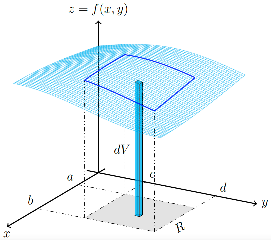
% A geometric representation of the differential of 
% volume in rectangular coordinates is shown.
% 
% Date of creation: September, 25th, 2021.
% Date of last modification: October, 9th, 2022.
% Author: Efraín Soto Apolinar.
% https://www.aprendematematicas.org.mx/author/efrain-soto-apolinar/instructing-courses/
% Source: page 121 of the 
% Glosario Ilustrado de Matem\'aticas Escolares.
% https://tinyurl.com/5udm2ufy
%
% Terms of use:
% According to TikZ.net
% https://creativecommons.org/licenses/by-nc-sa/4.0/
% Your commitment to the terms of use is greatly appreciated.
%
\begin{document}
%
\begin{center}
\tdplotsetmaincoords{70}{120}
%
\begin{tikzpicture}[tdplot_main_coords,scale=1.5]
    \tikzmath{function funcion(\x,\y) {return 2.5+0.25*sin((0.5*\x + \y) r);};}
    \pgfmathsetmacro{\step}{pi/50.0}
    \pgfmathsetmacro{\xi}{0}
    \pgfmathsetmacro{\xf}{1.0*pi}
    \pgfmathsetmacro{\xe}{\xf+\step}
    \pgfmathsetmacro{\xs}{\xi+\step}
    \pgfmathsetmacro{\yi}{0}
    \pgfmathsetmacro{\yf}{1.0*pi}
 
 
הההההההההההההההההההההההההההההההההההההההההההההההההההההההההההההההההההההההההההההההההההההההההההההההההההההההההההההההההההההההההההההההההההההההההההההההההההההההההההההההההההההההההההההההההההההההההההההההההההההההההההההההההההההההההההההההההההההההההההההההההההההההההההההההה
XXXXXXXXXXXXXXXXXXXXXXXXXXXXXXXXXXXXXXXXXXXXXXXXXXXXXXXXXXXXXXXXXXXXXXXXXXXXXXXXXXXXXXXXXXXXXXXXXXXXXXXXXXXXXXXXXXXXXXXXXXXXXXXXXXXXXXXXXXXXXXXXXXXXXXXXXXXXXXXXXXXXXXXXXXXXXXXXXXXXXXXXXXXXXXXXXXXXXXXXXXXXXXXXXXXXXXXXXXXXXXXXXXXXXXXXXXXXXXXXXXXXXXXXXXXXXXXX