")


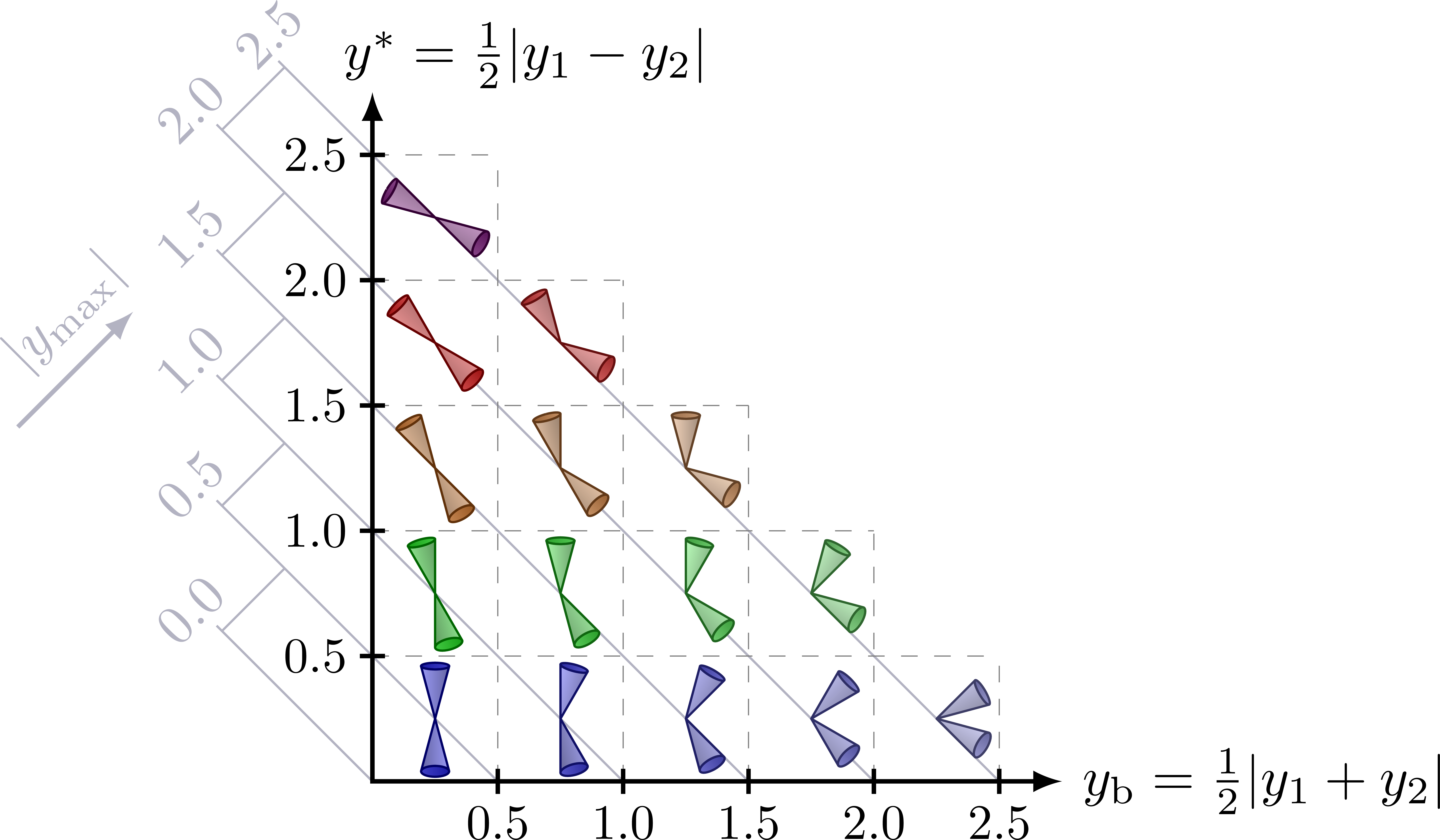
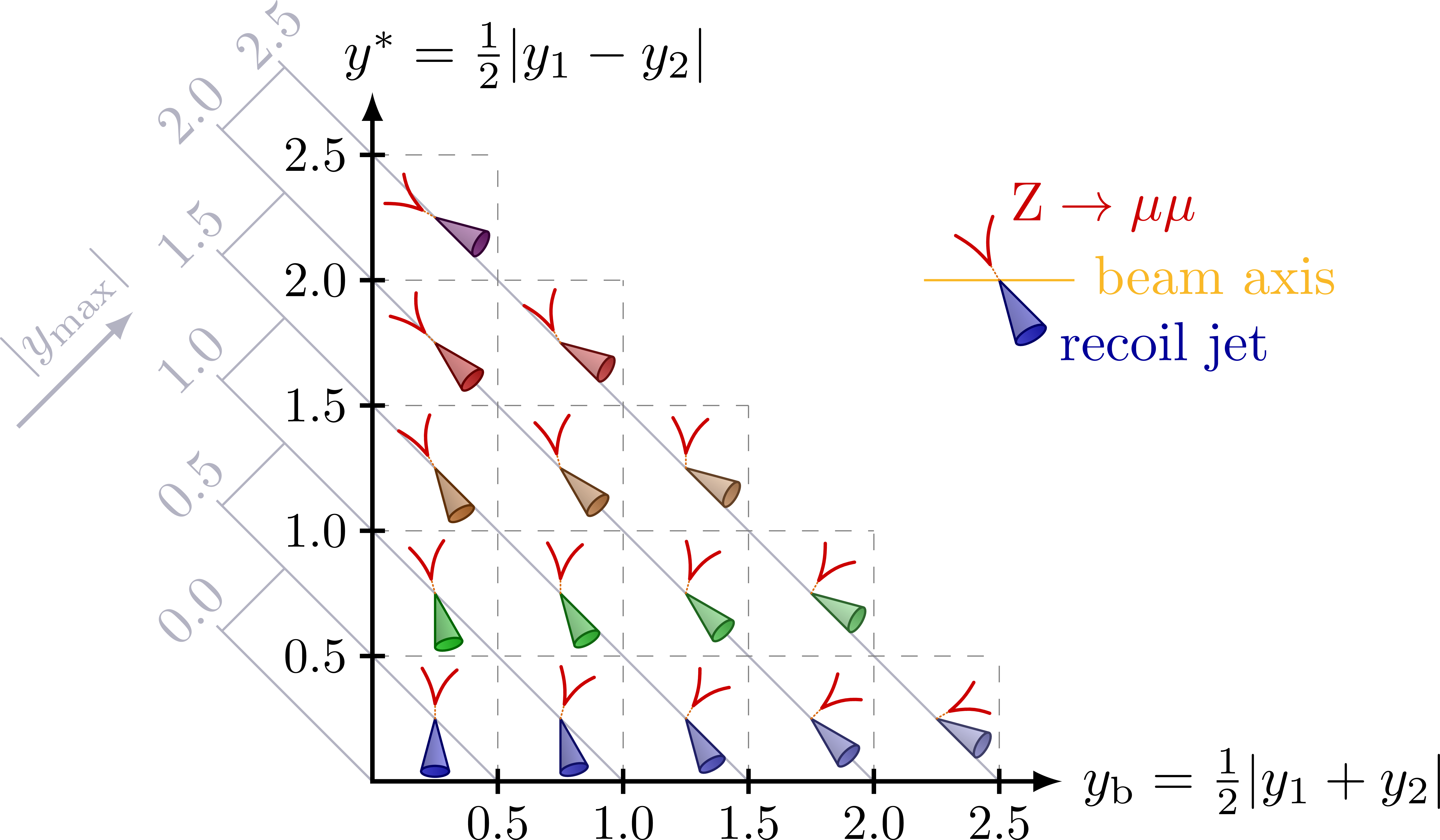
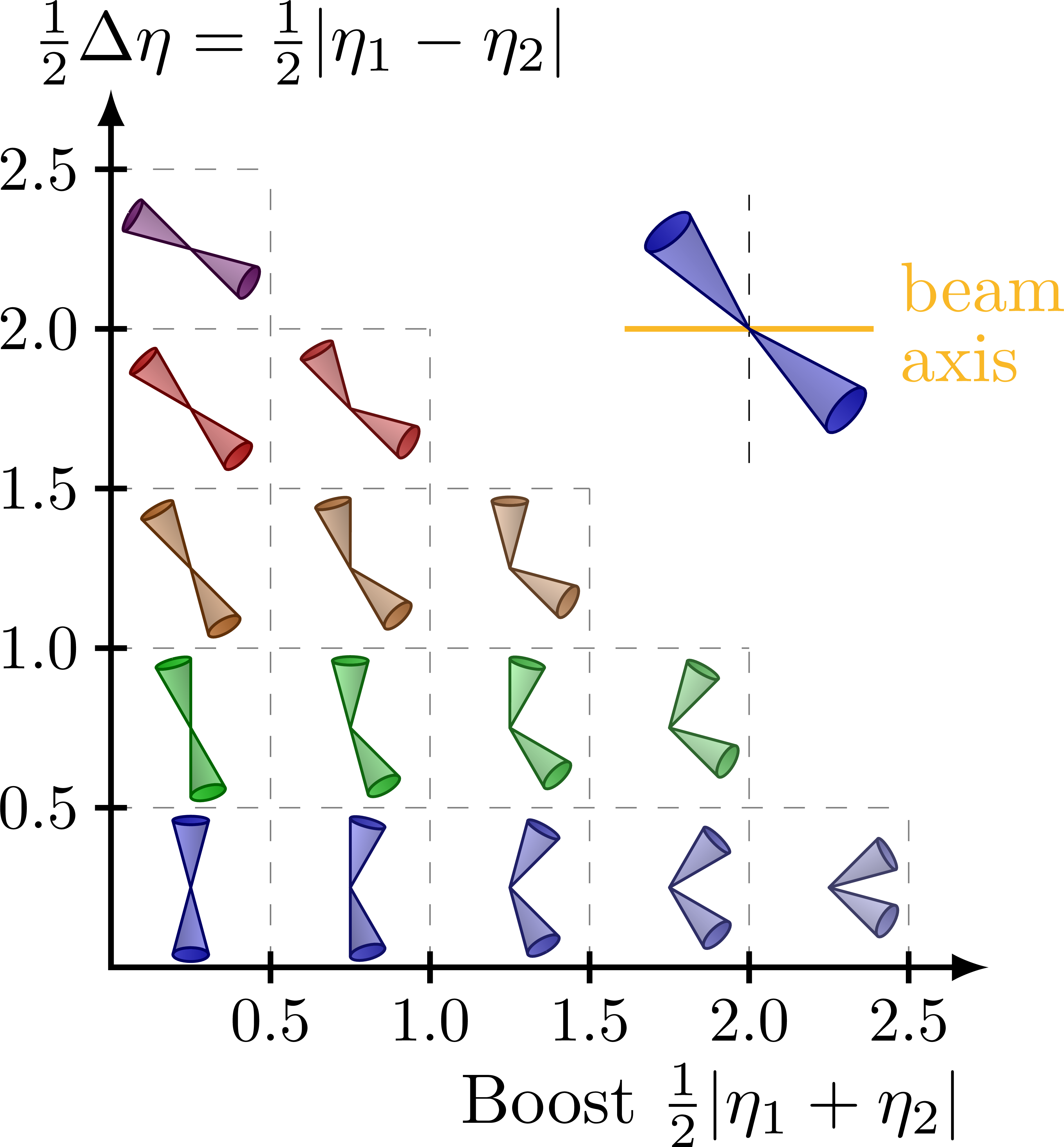
Different rapidity (y) regions of dijet and Z+jet events in terms of rapidity separation (y*) and boost (yb). For more related figures, please see the “jet” tag, or the Particle Physics category. The cones are constructed with the tangent methods presented here.
Dijet events (inspired by D. Savoiu’s PhD thesis; note that the dijets events shown below, assume Δφ = π):
Z → μμ recoiling against a jet (inspired by Dr. T. Berger’s PhD thesis):
Pseudorapidity η:
The basic for-loop for creating a matrix of arrows is
\documentclass[border=3pt,tikz]{standalone}
\begin{document}
\begin{tikzpicture}[scale=1.2]
  \def\N{7}
  \foreach \i [evaluate={\y=\i-0.5}] in {1,...,\N}{
    \foreach \j [evaluate={\x=\j-0.5;
                           \ang=80*(\i-1)/(\N-1); % seperation
                           \dang=90-70*(\j-1)/(\N-1); % boost
                 }] in {1,...,\N}{
      \draw[->,thick] (\x,\y) --++ (\ang-\dang:0.46); % bottom jet
      \draw[->,thick] (\x,\y) --++ (\ang+\dang:0.46); % top jet
      \fill[red] (\x,\y) circle(0.04);
    }
  }
\end{tikzpicture}
\end{document}
Edit and compile if you like:
% Author: Izaak Neutelings (October 2021)
% Description: Rapidity regions of dijet events
% Inspiration:
%   Daniel Savoiu, https://indico.cern.ch/event/1073619/#5-update-on-dijet-production-s
\documentclass[border=3pt,tikz]{standalone}
\usepackage{amsmath}
\usepackage{listofitems} % for \readlist to create arrays
\usepackage{xcolor}
\usepackage[outline]{contour} % glow around text
\usetikzlibrary{calc}
\usetikzlibrary{math} % for \tikzmath
\contourlength{1.0pt}
\tikzset{>=latex} % for LaTeX arrow head

\colorlet{myred}{red!80!black}
\colorlet{myblue}{blue!80!black}
\colorlet{mypurple}{blue!50!red}
\colorlet{myorange}{orange!90!red!95!black!90}
\colorlet{mydarkblue}{blue!60!black}
\colorlet{mygray}{blue!20!black!30}
\tikzstyle{muon}=[myred,line width=0.6,line cap=round]
\tikzstyle{boson}=[dash pattern=on 0.2 off 0.5,line width=0.3,line cap=round,myorange!90!black]
\readlist\cols{blue,green,myorange,red,mypurple} % list of colors

\newcommand\jetcone[5][blue]{{
  \pgfmathanglebetweenpoints{\pgfpointanchor{#2}{center}}{\pgfpointanchor{#3}{center}}
  \edef\ang{#4/2} % half-opening angle
  \edef\e{#5} % ratio a/b ("eccentricity") of cone top
  \edef\vang{\pgfmathresult} % angle of vector OV
  \tikzmath{
    coordinate \C;
    \C = (#2)-(#3); % vector OV
    \x = veclen(\Cx,\Cy)*\e*sin(\ang)^2; % x coordinate P
    \y = tan(\ang)*(veclen(\Cx,\Cy)-\x); % y coordinate P
    \a = veclen(\Cx,\Cy)*sqrt(\e)*sin(\ang); % vertical radius
    \b = veclen(\Cx,\Cy)*tan(\ang)*sqrt(1-\e*sin(\ang)^2); % horizontal radius
    \angb = acos(sqrt(\e)*sin(\ang)); % angle of P in ellipse
  }
  \coordinate (tmpL) at ($(#3)-(\vang:\x pt)+(\vang+90:\y pt)$); % tangency
  \draw[thin,#1!40!black,rotate=\vang, %,fill=#1!50!black!80
    top color=#1!60!black!90,bottom color=#1!70!black!75,shading angle=\vang]
    (#3) ellipse({\a pt} and {\b pt});
  \draw[thin,#1!40!black,rotate=\vang,rounded corners=0.03,
  top color=#1!90!black!40,bottom color=#1!40!black!60,shading angle=\vang]
    (tmpL) arc(180-\angb:180+\angb:{\a pt} and {\b pt})
    -- (#2) -- cycle;
}}
\def\tick#1#2{\draw[thick] (#1) ++ (#2:0.1) --++ (#2-180:0.2)}


\begin{document}


% DIJET EVENTS
% Daniel Savoiu, https://indico.cern.ch/event/1073619/#5-update-on-dijet-production-s
\begin{tikzpicture}[scale=0.8]

  \def\N{5} % number of eta bins with width 0.5

  % DIAGONAL GRIDS (ymax)
  \foreach \i [evaluate={\ym=0.5*(\i-1);}] in {1,...,\N}{
    \draw[mygray]
      (\i-1,0) --++ (135:{sqrt(2)*(\i+0.2)}) coordinate (T\i) --++ (45:{sqrt(2)/2});
    \draw[mygray] (T\i) --++ (135:0.06) node[above=-2,rotate=45] {\ym};
  }
  \draw[mygray] (\N,0) --++ (135:{sqrt(2)*(\N+0.75)}) node[right=3,above=0,rotate=45] {2.5};

  % GRIDS
  \foreach \i [evaluate={\y=\i-0.5; \Nx=\N-\i+1; \e=0.5*\i}] in {1,...,\N}{
    \draw[very thin,dashed,black!50] (0,\i) --++ (\Nx,0);
    \draw[very thin,dashed,black!50] (\i,0) --++ (0,\Nx);
    \tick{0,\i}{0} node[left=-1,scale=0.9] {\e};
    \tick{\i,0}{90} node[below=-1,scale=0.9] {\e};
  }

  % JETS
  \foreach \i [evaluate={\y=\i-0.5; \Nx=\N-\i+1; \e=0.5*\i}] in {1,...,\N}{
    \foreach \j [evaluate={\x=\j-0.5; \mix=100-60*(\j-1)/(\N-1);
                           \ang=60*(\i-1)/(\N-1); % seperation
                           \dang=90-60*(\j-1)/(\N-1); % boost
                 }] in {1,...,\Nx}{
      \colorlet{conecol}{\cols[\i]!\mix} % color for cone
      \coordinate (O) at (\x,\y); % primary vertex
      \coordinate (T) at ($(\x,\y)+(\ang+\dang:0.42)$); % top jet
      \coordinate (B) at ($(\x,\y)+(\ang-\dang:0.42)$); % bottom jet
      \jetcone[conecol]{O}{T}{30}{0.06} %!70!white
      \jetcone[conecol]{O}{B}{30}{0.16}
    }
  }

  % AXIS
  \draw[<->,thick]
    (0,1.1*\N) %node[left] {\contour{white}{$y*$}} --
    node[left=6,above right=-3] {$y^* = \frac{1}{2}|y_1-y_2|$} --
    (0,0) -- (1.1*\N,0) node[right] {$y_\text{b} = \frac{1}{2}|y_1+y_2|$};
  \draw[->,thick,mygray]
    (135:4.0) --++ (45:1.3)
    node[pos=0.7,above,rotate=45] {$|y_\text{max}|$};

\end{tikzpicture}


% Z -> mumu recoil against jet
% Thomas Berge, https://publish.etp.kit.edu/record/21710
\begin{tikzpicture}[scale=0.8]

  \def\N{5} % number of eta bins with width 0.5

  % DIAGONAL GRIDS (ymax)
  \foreach \i [evaluate={\ym=0.5*(\i-1);}] in {1,...,\N}{
    \draw[mygray]
      (\i-1,0) --++ (135:{sqrt(2)*(\i+0.2)}) coordinate (T\i) --++ (45:{sqrt(2)/2});
    \draw[mygray] (T\i) --++ (135:0.06) node[above=-2,rotate=45] {\ym};
  }
  \draw[mygray] (\N,0) --++ (135:{sqrt(2)*(\N+0.75)}) node[right=3,above=0,rotate=45] {2.5};

  % GRIDS
  \foreach \i [evaluate={\y=\i-0.5; \Nx=\N-\i+1; \e=0.5*\i}] in {1,...,\N}{
    \draw[very thin,dashed,black!50] (0,\i) --++ (\Nx,0);
    \draw[very thin,dashed,black!50] (\i,0) --++ (0,\Nx);
    \tick{0,\i}{0} node[left=-1,scale=0.9] {\e};
    \tick{\i,0}{90} node[below=-1,scale=0.9] {\e};
  }

  % JETS
  \foreach \i [evaluate={\y=\i-0.5; \Nx=\N-\i+1; \e=0.5*\i}] in {1,...,\N}{
    \foreach \j [evaluate={\x=\j-0.5; \mix=100-60*(\j-1)/(\N-1);
                           \ang=60*(\i-1)/(\N-1); % seperation
                           \dang=90-60*(\j-1)/(\N-1); % boost
                 }] in {1,...,\Nx}{
      \colorlet{conecol}{\cols[\i]!\mix} % color for cone
      \coordinate (O) at (\x,\y); % primary vertex
      \coordinate (T) at ($(\x,\y)+(\ang+\dang:0.12)$); % Z -> mumu
      \coordinate (B) at ($(\x,\y)+(\ang-\dang:0.42)$); % jet cone
      \jetcone[conecol]{O}{B}{30}{0.16}
      \draw[boson] (O) -- (T);
      \draw[muon] (T) to[out=\ang+\dang+10,in=\ang+\dang-150]++ (\ang+\dang+20:0.30);
      \draw[muon] (T) to[out=\ang+\dang-20,in=\ang+\dang+130]++ (\ang+\dang-33:0.32);
    }
  }

  % LEGEND
  \begin{scope}[shift={(5,4)},scale=1.2]
    \def\ang{120}
    \coordinate (O) at (0,0); % primary vertex
    \coordinate (T) at (\ang:0.12); % muons
    \coordinate (B) at (\ang+180:0.42); % jet cone
    %\colorlet{conecol}{\cols[0]} % color for cone
    \draw[myorange!60!yellow!90,thin] (-0.5,0) -- (0.5,0)
      node[above=1,right,scale=1] {beam axis};
    \jetcone[blue]{O}{B}{30}{0.16}
    \draw[boson] (O) -- (T);
    \draw[muon] (T) to[out=\ang+10,in=\ang-150]++ (\ang+20:0.30);
    \draw[muon] (T) to[out=\ang-20,in=\ang+130]++ (\ang-33:0.32) coordinate (M);
    \node[anchor=185,inner sep=3,myred,scale=1] at (M) {$\mathrm{Z}\to\mu\mu$};
    \node[anchor=175,inner sep=5,mydarkblue,scale=1] at (B) {recoil jet};
  \end{scope}

  % AXIS
  \draw[<->,thick]
    (0,1.1*\N) %node[left] {\contour{white}{$y*$}} --
    node[left=6,above right=-3] {$y^* = \frac{1}{2}|y_1-y_2|$} --
    (0,0) -- (1.1*\N,0) node[right] {$y_\text{b} = \frac{1}{2}|y_1+y_2|$};
  \draw[->,thick,mygray]
    (135:4.0) --++ (45:1.3)
    node[pos=0.7,above,rotate=45] {$|y_\text{max}|$};

\end{tikzpicture}


% DIJET EVENTS - PSEUDORAPIDITY
% Daniel Savoiu, https://indico.cern.ch/event/1073619/#5-update-on-dijet-production-s
\begin{tikzpicture}[scale=0.8]

  \def\N{5} % number of eta bins with width 0.5

  %% DIAGONAL GRIDS (ymax)
  %\foreach \i [evaluate={\ym=0.5*(\i-1);}] in {1,...,\N}{
  %  \draw[mygray]
  %    (\i-1,0) --++ (135:{sqrt(2)*(\i+0.2)}) coordinate (T\i) --++ (45:{sqrt(2)/2});
  %  \draw[mygray] (T\i) --++ (135:0.06) node[above=-2,rotate=45] {\ym};
  %}
  %\draw[mygray] (\N,0) --++ (135:{sqrt(2)*(\N+0.75)}) node[right=3,above=0,rotate=45] {2.5};

  % GRIDS
  \foreach \i [evaluate={\y=\i-0.5; \Nx=\N-\i+1; \e=0.5*\i}] in {1,...,\N}{
    \draw[very thin,dashed,black!50] (0,\i) --++ (\Nx,0);
    \draw[very thin,dashed,black!50] (\i,0) --++ (0,\Nx);
    \tick{0,\i}{0} node[left=-1,scale=0.9] {\e};
    \tick{\i,0}{90} node[below=-1,scale=0.9] {\e};
  }

  % JETS
  \foreach \i [evaluate={\y=\i-0.5; \Nx=\N-\i+1; \e=0.5*\i}] in {1,...,\N}{
    \foreach \j [evaluate={\x=\j-0.5; \mix=100-60*(\j-1)/(\N-1);
                           \ang=60*(\i-1)/(\N-1); % seperation
                           \dang=90-60*(\j-1)/(\N-1); % boost
                 }] in {1,...,\Nx}{
      \colorlet{conecol}{\cols[\i]!\mix} % color for cone
      \coordinate (O) at (\x,\y); % primary vertex
      \coordinate (T) at ($(\x,\y)+(\ang+\dang:0.42)$); % top jet
      \coordinate (B) at ($(\x,\y)+(\ang-\dang:0.42)$); % bottom jet
      \jetcone[conecol]{O}{T}{30}{0.06} %!70!white
      \jetcone[conecol]{O}{B}{30}{0.16}
    }
  }

  % AXIS
  \draw[<->,thick]
    (0,1.1*\N) %node[left] {\contour{white}{$y*$}} --
    node[left=12,above right=-3] {$\frac{1}{2}\Delta\eta = \frac{1}{2}|\eta_1-\eta_2|$} --
    (0,0) -- (1.1*\N,0) node[yshift=-10pt,below left=0pt] {Boost $\frac{1}{2}|\eta_1+\eta_2|$}; %\eta_\text{b} =
  %\draw[->,thick,mygray]
  %  (135:4.0) --++ (45:1.3)
  %  node[pos=0.7,above,rotate=45] {$|\eta_\text{max}|$};


  % LEGEND
  \begin{scope}[shift={(4,4)},scale=1.2]
    \coordinate (O) at (0,0); % primary vertex
    \coordinate (T) at (130:0.66); % muons
    \coordinate (B) at (-40:0.66); % jet cone
    %\colorlet{conecol}{\cols[0]} % color for cone
    \draw[dashed,very thin] (0,-0.7) -- (0,0.7);
    \draw[myorange!60!yellow!90,thick] (-0.65,0) -- (0.65,0)
      node[above=1,right,scale=1,align=left] {beam\\[-2pt]axis};
    %\draw[boson] (O) -- (T);
    \jetcone[blue]{O}{T}{25}{0.16}
    \jetcone[blue]{O}{B}{25}{0.16}
    %\draw[->,thick,myblue] (O) -- (T);
    %\draw[->,thick,myblue] (O) -- (B);
    %\node[anchor=185,inner sep=3,myred,scale=0.9] at (T) {$\mathrm{Z}\to\mu\mu$};
    %\node[anchor=175,inner sep=5,mydarkblue,scale=0.9] at (B) {recoil jet};
  \end{scope}

\end{tikzpicture}


\end{document}
Click to download: jet_eta.tex • jet_eta.pdf
Open in Overleaf: jet_eta.tex


