")


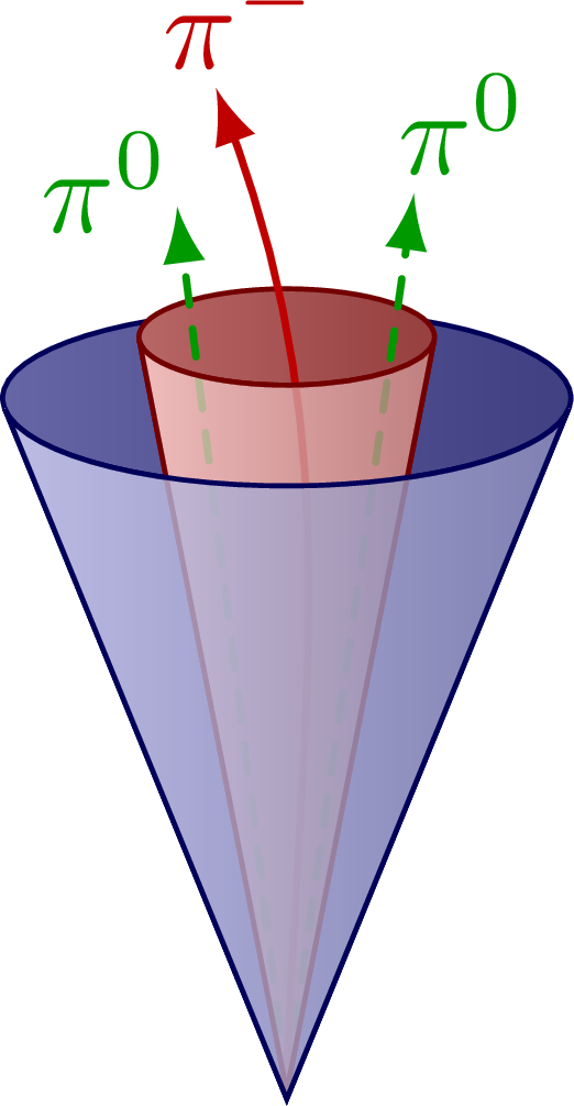
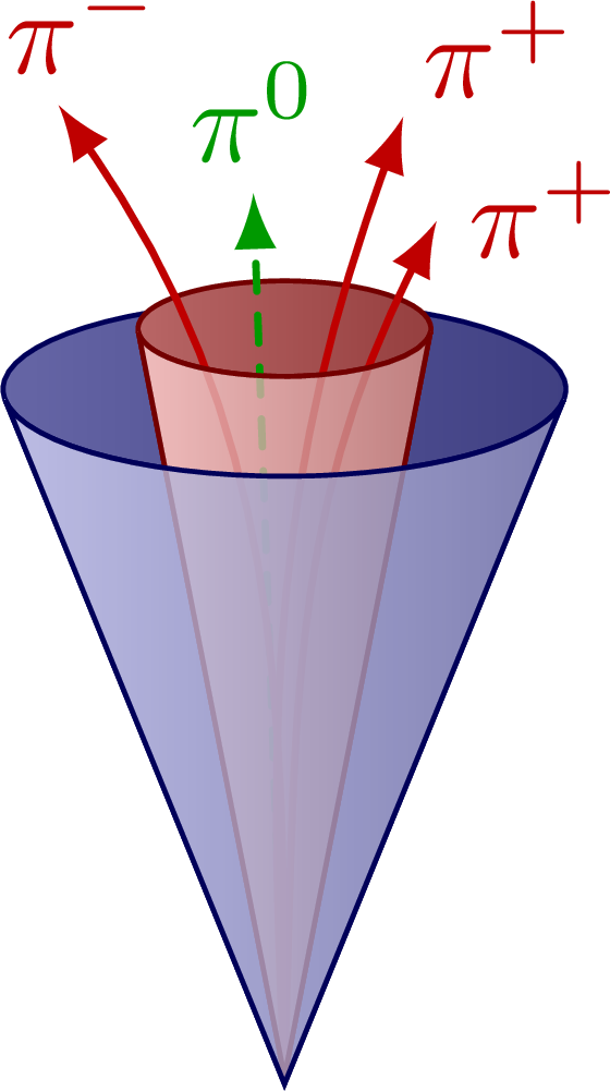
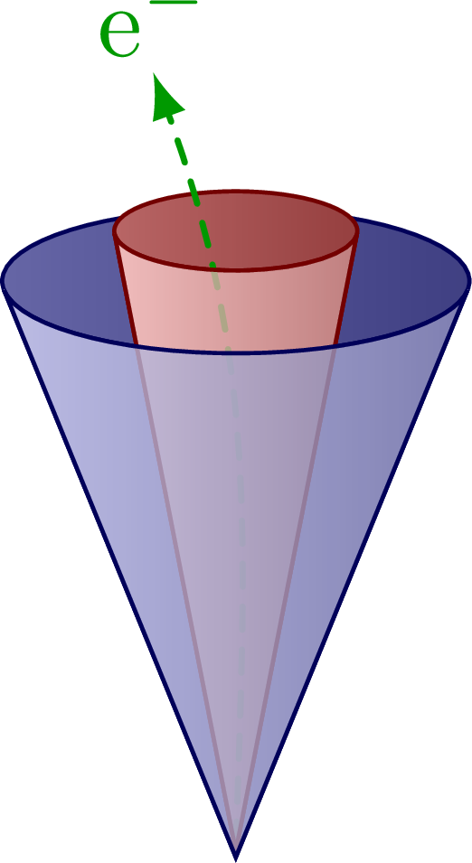
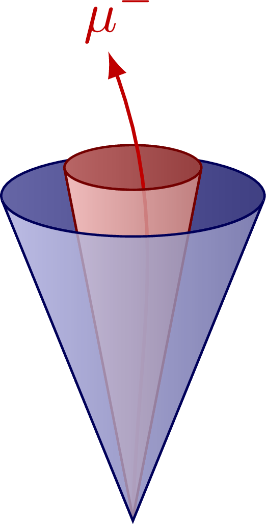
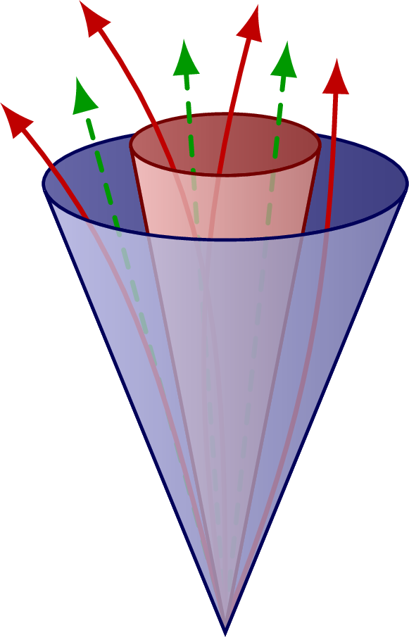
Isolation (blue) and signal cone (red) of a hadronically decayed tau, and for comparison an electron, muon and quark/gluon-initiated jet. For more related figures, please see the “jet” tag or the Particle Physics category. The cones are constructed with the tangent methods presented here. The neutrinos from τ decay are invisible to the detector and are not shown in the illustrations below.
A hadronic jet initiated by a τ lepton that decays to a charge pion (“one prong”), and two neutral pions (π0s):
A hadronic jet initiated by a τ lepton that decays to three charge pions (“three prong”) plus one π0:
An isolated electron, that may be misidentified as a τ lepton decay to a single charged pion (“one prong”):
An isolated muon, that may be misidentified as a τ lepton decay to a single charged pion (“one prong”):
A hadronic jet initiated by a quark or gluon, which tend to have more activity in the isolation cone:
Edit and compile if you like:
% Author: Izaak Neutelings (November 2021)
% Description: jet cones for taus & others
\documentclass[border=3pt,tikz]{standalone}
\usetikzlibrary{calc}
\usetikzlibrary{math} % for \tikzmath
\tikzset{>=latex} % for LaTeX arrow head

\colorlet{myblue}{blue!70!black}
%\colorlet{mydarkblue}{blue!50!black}
\colorlet{mygreen}{green!60!black}
\colorlet{myred}{red!75!black}
\colorlet{isocol}{blue!70!black} % color isolation cone
\colorlet{sigcol}{red!90!black} % color isolation cone
\tikzstyle{track}=[->,line width=0.6,myred]
\tikzstyle{dashed track}=[->,mygreen,line width=0.6,line cap=round,
                          dash pattern=on 2.3 off 2.0]

\newcommand\jetcone[6][sigcol]{{
  \pgfmathanglebetweenpoints{\pgfpointanchor{#2}{center}}{\pgfpointanchor{#3}{center}}
  \pgfmathsetmacro\oang{#4/2} % half-opening angle
  \edef\e{#5} % ratio a/b
  \def\tmpL{tmpL-#2-#3} % unique coordinate name
  \edef\vang{\pgfmathresult} % angle of vector OV
  \tikzmath{
    coordinate \C;
    \C = (#2)-(#3);
    \x = veclen(\Cx,\Cy)*\e*sin(\oang)^2; % x coordinate P
    \y = tan(\oang)*(veclen(\Cx,\Cy)-\x); % y coordinate P
    \a = veclen(\Cx,\Cy)*sqrt(\e)*sin(\oang); % vertical radius
    \b = veclen(\Cx,\Cy)*tan(\oang)*sqrt(1-\e*sin(\oang)^2); % horizontal radius
    \angb = acos(sqrt(\e)*sin(\oang)); % angle of P in ellipse
  }
  \coordinate (\tmpL) at ($(#3)-(\vang:\x pt)+(\vang+90:\y pt)$); % tangency
  \draw[thin,#1!50!black,fill=#1!80!black!50,rotate=\vang] % cone back
    (\tmpL) arc(180-\angb:180+\angb:{\a pt} and {\b pt})
    -- ($(#2)+(0.01,0)$) -- cycle;
  \draw[thin,#1!50!black,rotate=\vang, % cone inside
        top color=#1!60!black!60,bottom color=#1!50!black!75,shading angle=\vang]
    (#3) ellipse({\a pt} and {\b pt});
  #6 % extra tracks
  \draw[thin,#1!50!black,rotate=\vang,fill opacity=0.80, % cone front
        top color=#1!90!black!20,bottom color=#1!50!black!50,shading angle=\vang]
    (\tmpL) arc(180-\angb:180+\angb:{\a pt} and {\b pt})
    -- ($(#2)+(0.01,0)$) -- cycle;
}}


\begin{document}

% COMMON SETTINGS
\small
\def\angiso{44} % opening angle of isolation cone
\def\angsig{22} % opening angle of isolation cone
\def\e{0.11}    % a/b ratio of ellipse minor and major radii

\foreach \ang [evaluate={\ang; \anang=\ang-90;}] in {90,\angiso/2,0,180}{ % rotate each cone
  \tikzset{
    every picture/.append style={scale=2.4,rotate=\ang-90}, % set scale for all figures
    every node/.style={inner sep=1,circle} %,draw=black!9,very thin}
  }


  % TAU JET - ONE PRONG
  \begin{tikzpicture}
    \coordinate (O)  at (0,0);
    \coordinate (O') at (0,-0.01); % shifted
    \coordinate (I)  at (0,0.92); % isolation cone
    \coordinate (S)  at (0,1.00); % signal cone
    \coordinate (T)  at (0,0.02); % tau vertex
    \jetcone[isocol]{O'}{I}{\angiso}{\e}{ % isolation cone
      \jetcone[sigcol]{O}{S}{\angsig}{\e}{ % signal cone
        \draw[track] (T) to[out=88,in=-70] (93:1.33)
          node[anchor=-70+\anang,inner sep={2.5*cos(\ang)^2-1.5}] {$\pi^-$};
      }
    }
  \end{tikzpicture}


  % TAU JET - ONE PRONG, 2 PI ZEROS
  \begin{tikzpicture}
    \jetcone[isocol]{O'}{I}{\angiso}{\e}{ % isolation cone
      \jetcone[sigcol]{O}{S}{\angsig}{\e}{ % signal cone
        \draw[dashed track] (T) -- (97:1.18)
          node[anchor=-40+\anang,inner sep={2*cos(\ang)^2-1.0}] {$\pi^0$};
        \draw[dashed track] (T) -- (82:1.20)
          node[anchor=-110+\anang,inner sep=0.0] {$\pi^0$};
        \draw[track] (T) to[out=88,in=-70] (94:1.33)
          node[anchor=-100+\anang,inner sep={-sin(\ang)^2}] {$\pi^-$};
      }
    }
  \end{tikzpicture}


  % TAU JET - THREE PRONG
  \begin{tikzpicture}
    \jetcone[isocol]{O'}{I}{\angiso}{\e}{ % isolation cone
      \jetcone[sigcol]{O}{S}{\angsig}{\e}{ % signal cone
        \draw[track] (T) to[out=90,in=-55] (103:1.33)
          node[anchor=-70+\anang,inner sep={2.5*cos(\ang)^2-1.5}] {$\pi^-$};
        \draw[track] (T) to[out=90,in=-112] (87:1.29)
          node[anchor=-110+\anang,inner sep={0.6*sin(\ang)^2}] {$\pi^+$};
        \draw[track] (T) to[out=88,in=-117] (82:1.16)
          node[anchor=-145+\anang,inner sep={0.6*sin(\ang)^2}] {$\pi^+$};
      }
    }
  \end{tikzpicture}


  % TAU JET - THREE PRONG, PI ZERO
  \begin{tikzpicture}
    \jetcone[isocol]{O'}{I}{\angiso}{\e}{ % isolation cone
      \jetcone[sigcol]{O}{S}{\angsig}{\e}{ % signal cone
        \draw[dashed track] (T) -- (92:1.18)
          node[anchor=-85+\anang,inner sep=0.5] {$\pi^0$};
        \draw[track] (T) to[out=90,in=-55] (103:1.33)
          node[anchor=-70+\anang,inner sep={2.5*cos(\ang)^2-1.5}] {$\pi^-$};
        \draw[track] (T) to[out=93,in=-110] (84:1.29)
          node[anchor=-110+\anang,inner sep={0.6*sin(\ang)^2}] {$\pi^+$};
        \draw[track] (T) to[out=88,in=-117] (80:1.16)
          node[anchor=-145+\anang,inner sep={0.6*sin(\ang)^2}] {$\pi^+$};
      }
    }
  \end{tikzpicture}


  % ELECTRON JET
  \begin{tikzpicture}
    \jetcone[isocol]{O'}{I}{\angiso}{\e}{ % isolation cone
      \jetcone[sigcol]{O}{S}{\angsig}{\e}{ % signal cone
        %\draw[dashed track] (T) to[out=88,in=-70] (96:1.26)
        %  node[right=0,above=-2] {$\mathrm{e}^-$};
        \draw[dashed track] (T) to[out=88,in=-70] (96:1.26)
          node[anchor=-70+\anang,inner sep={2.5*cos(\ang)^2-1.5}]  {$\mathrm{e}^-$};
      }
    }
  \end{tikzpicture}


  % MUON JET
  \begin{tikzpicture}
    \jetcone[isocol]{O'}{I}{\angiso}{\e}{ % isolation cone
      \jetcone[sigcol]{O}{S}{\angsig}{\e}{ % signal cone
        \draw[track] (T) to[out=88,in=-70] (93:1.33)
          node[anchor=-70+\anang,inner sep={2.5*cos(\ang)^2-1.5}] {$\mu^-$};
      }
    }
  \end{tikzpicture}


  % QUARK/GLUON JET
  \begin{tikzpicture}
    \jetcone[isocol]{O'}{I}{\angiso}{\e}{ % isolation cone
      \jetcone[sigcol]{O}{S}{\angsig}{\e}{ % signal cone
        \draw[dashed track] (T) -- (105:1.18);
        \draw[dashed track] (T) -- (94:1.22);
        \draw[dashed track] (T) -- (84:1.22);
        \draw[track] (T) to[out=105,in=-50] (113:1.18);
        \draw[track] (T) to[out=90,in=-55] (103:1.33);
        \draw[track] (T) to[out=98,in=-105] (87:1.29);
        \draw[track] (T) to[out=68,in=-92] (79:1.20);
      }
    }
  \end{tikzpicture}


} % end \foreach


\end{document}
Click to download: jet_tau.tex • jet_tau.pdf
Open in Overleaf: jet_tau.tex

 production")

