")


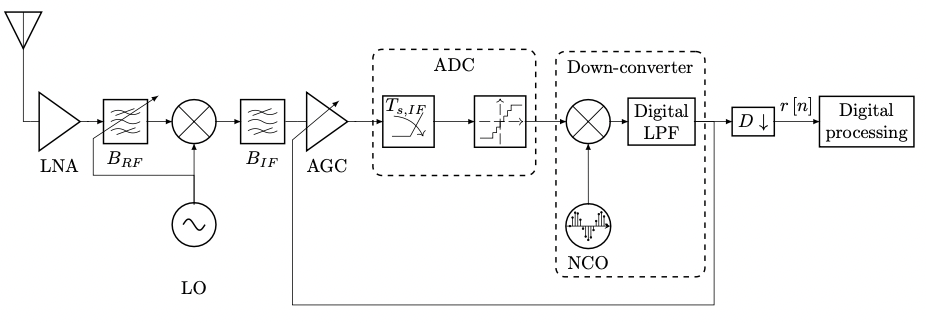
This is an example of a block diagram of a radiofrequency front-end (RF-FE).
\documentclass[border=10pt]{standalone}
\usepackage{tikz}
\usepackage{pgfplots} % loads tikz which loads pgf
\usepackage[american,siunitx]{circuitikz}
\usetikzlibrary{arrows,calc,positioning,fit}
\pgfplotsset{
  compat=1.15,
  within block/.style={
    scale only axis,
    scale=0.423,
    anchor=center,
    axis x line=middle,
    axis y line=none,
    enlargelimits=0.1,
    width=2cm,
    height=15mm,
    xtick=\empty,
    ytick=\empty,
    domain=0:85,
    samples=15,
    tickwidth=0,
    clip mode=individual,
    every axis plot/.append style={
        smooth,
        mark options={
            draw=black,
            fill=black,
            mark size=1pt
        }
    },
    before end axis/.code={
        \node [draw,thick, shape=circle, inner sep=-2pt,
          fit=(current axis), label={below:{NCO}}] (nco) {};
        }
    }
}

\newcommand{\mixer}[2]
{  % #1 = reference coordinate, #2 = name
  \node[draw, thick, shape=circle, minimum size=24pt, at={#1}](#2){};
  \draw[rotate=45,line width=0.5pt] (#2.center)+(0,-12pt) -- +(0,12pt);
  \draw[rotate=-45,line width=0.5pt] (#2.center)+(0,-12pt) -- +(0,12pt);
}

\newcommand{\BPF}[3]
{ % #1 - reference coordinate, #2 - name, #3 - subscript label
    \node[
        draw,
        shape=rectangle,
        thick,
        minimum size=24pt,
        at={#1},
        label={below:{#3}}
    ](#2){};

    %%% middle tilde
    \draw (#2.center)+(-8pt,0) % first coordinate for the line segment
        to[bend left] (#2.center) % draw a curved line that bends to the left. The curve starts at the first coordinate and ends at the next coordinate.
        to[bend right] +(8pt,0); % This means to draw a curved line that bends to the right. The curve starts at the previous coordinate and ends at the next coordinate.
    %%% upper tilde
    \draw ([yshift=5pt]#2.center)+(-8pt,0) % starting point of the path. The yshift key is used to shift the starting point vertically by 5pt.
        to[bend left] ([yshift=5pt]#2.center) % second point of the path. It is located at the center of the bpf node, shifted 5pt vertically.
        to[bend right] +(8pt,0); % third point of the path. It is located 8pt to the right, relative to the second point. The + sign indicates that the point is relative to the second control point.
    \draw[rotate=20] ([yshift=5pt]#2.center)+(-4pt,0) -- +(7pt,0); % strike out the upper tilde
    %%% lower tilde
    \draw ([yshift=-5pt]#2)+(-8pt,0)
        to[bend left] ([yshift=-5pt]#2.center)
        to[bend right] +(8pt,0);
    \draw[rotate=20] ([yshift=-5pt]#2.center) +(-7pt,0) -- +(4pt,0);
}

\newcommand{\ADC}[2]{
\begin{scope}[transform shape,rotate=#2]
    %%% sampler
    \node[draw, shape=rectangle, thick, minimum width=28pt, minimum height=28pt, at={(#1)}](sampler){};
    \draw (sampler.center)+(-9pt,-8pt)
        to +(1pt,-8pt)
        to +(8pt,5pt);
    \draw[->] (sampler.center)+(-8pt,3pt)
        node[shift={(7pt,5pt)}]() {\(T_{s,IF}\)}
        to[bend left] +(8pt,-8pt);

    %%% quantizer
    \node[draw, shape=rectangle, thick, minimum size=28pt, at={([xshift=50pt]sampler)}](quantizer){}; % rectangle
    \draw[->, line width=0.1pt, dashed, dash pattern= on 6pt off 2pt] ($(quantizer.south)+(0pt,+2pt)$) -- ($(quantizer.north)+(0pt,-2pt)$); % axis
    \draw[->, line width=0.1pt, dashed, dash pattern= on 6pt off 2pt] ($(quantizer.west)+(3pt,0pt)$) -- ($(quantizer.east)+(-2pt,0pt)$);
    \coordinate (begin) at ($(quantizer.center)+(-6pt,-9pt)$); % steps
    \foreach \i in {0,...,5} {
        \ifnum \i=0
            \draw (begin)+(-5pt,0pt) -- (begin) -- +(2pt,0pt) -- +(2pt,3pt);
        \else
            \ifnum \i=5
                \draw ($(begin)+\i*(2pt,3pt)$) -- +(2pt,0pt) -- +(2pt,3pt) -- +(8pt,3pt);
            \else
                \draw ($(begin)+\i*(2pt,3pt)$) -- +(2pt,0pt) -- +(2pt,3pt);
            \fi
        \fi
    }

    %%% ADC (outside block)
    \node[draw, fit=(sampler) (quantizer), thick, rounded corners=5pt, inner ysep=20pt, inner xsep=5pt, yshift=5pt, dashed](adc-fit){};
    \node[below, inner sep=5pt] at (adc-fit.north) {ADC};
\end{scope}
}

\tikzset{ar/.style={-latex,shorten >=-1pt, shorten <=-1pt}}
\begin{document}

\begin{circuitikz}

%%% antenna
\node[shape=antenna, xscale=-1, at={(-0.5,3)}](antenna){};

%%% LNA
\draw ([xshift=20pt]antenna.south) % starts a new drawing command at coordinate (0,3)
    node[shape=buffer,scale=0.8](lna){} % adds a node at the current coordinate with the shape buffer and a scaling factor of 0.8. The lna label is assigned to this node, which can be used later to reference it.
    node[below=0.6cm]{LNA}; %  adds a label "LNA" above the buffer node, positioned 0.8 cm above the node's center.

%%% RF BPF
\BPF{([xshift=20pt]lna.out)}{rf-bpf}{\(B_{RF}\)}

%%% mixer1
\mixer{([xshift=25pt]rf-bpf.east)}{mixer1}

%%% IF BPF
\BPF{([xshift=25pt]mixer1.east)}{if-bpf}{\(B_{IF}\)}

%%% LO
\path (mixer1.center)
    to[midway, sV, name=lo]
    node[at={(lo.south)}](){LO}
    ([yshift=-100pt]mixer1.south);

%%% AGC
\draw (if-bpf.east)+(0.8,0) % starts a new drawing command at coordinate (0,3)
    node[shape=buffer,scale=0.8](agc){} % adds a node at the current coordinate with the shape buffer and a scaling factor of 0.8. The lna label is assigned to this node, which can be used later to reference it.
    node[below=0.6cm]{AGC}; %  adds a label "LNA" above the buffer node, positioned 0.8 cm above the node's center.

%%% ADC
\path (agc.out)+(2,0)
    to[sV,color=white,name=adc]
    (agc.out)+(3,0);
\ADC{adc.center}{0}

%%% mixer2
\mixer{([xshift=110pt]adc.east)}{mixer2}

%%% NCO
\begin{axis}[ % no position defined, so this ends up at (0,0)
    within block=ax1,
    at={($(mixer2.center)+(-12pt,-48pt)$)},
    anchor=north west]
    \addplot+[
        ycomb,
        black,
        mark options={
            draw=black,
            fill=black,
            mark size=1pt
        },
    ]  {sin(2*pi*x)};
\end{axis}


%%% digital LPF
\node[draw, thick, shape=rectangle, minimum size=12pt, at={([xshift=40pt]mixer2.center)}, align=center](digital-lpf){Digital\\LPF};

%%% down-converter (outside block)
\node[draw, fit=(nco) (digital-lpf), thick, rounded corners=5pt, inner ysep=20pt, inner xsep=5pt, yshift=5pt, dashed](down-converter){};
\node[below, inner sep=5pt] at (down-converter.north) {Down-converter};

%%% decimator
\node[draw, thick, shape=rectangle, minimum size=12pt, at={([xshift=50pt]digital-lpf.center)}, align=center](decimator){$D \downarrow$};

%%% digital processing
\node[draw, thick, shape=rectangle, minimum size=12pt, at={([xshift=50pt]decimator.east)}, align=center](digital-processing){Digital\\processing};

%%% wiring
\draw[] (antenna.south) -- (lna.in);
\draw[ar] (lna.out)--(rf-bpf);
\draw[ar] (rf-bpf)--(mixer1);
\draw[ar] (lo.west)--(mixer1); % `lo' is rotated, `lo.west' actually means its top
\draw[ar] (lo.west)-- +(0pt,15pt) |- +(-55pt,15pt) |- +(-55pt,35pt) -- +(-20pt,58pt);
\draw[ar] (mixer1) -- (if-bpf);
\draw[] (if-bpf) -- (agc.in);
\draw[ar] (agc.out) -- (sampler.west);
\draw[ar] (sampler.east) -- (quantizer.west);
\draw[ar] (quantizer.east) -- (mixer2.west);
\draw[ar] (nco.north) -- (mixer2.south);
\draw[ar] (mixer2.east) -- (digital-lpf.west);
\draw[ar] (digital-lpf.east) -- (decimator.west);
\draw[ar] (digital-lpf.east) -- +(10pt,0pt) |- +(0pt,-100pt) -- +(-220pt,-100pt) -- +(-220pt,-10pt) -- ([yshift=-5pt, xshift=6pt]agc.north);
\draw[ar] (decimator.east) --
    node[pos=0.5, above]() {\(r\left[ n \right]\)}
    (digital-processing.west);
\end{circuitikz}
\end{document}