Event classification with jets

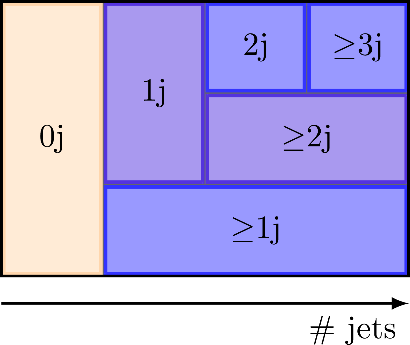
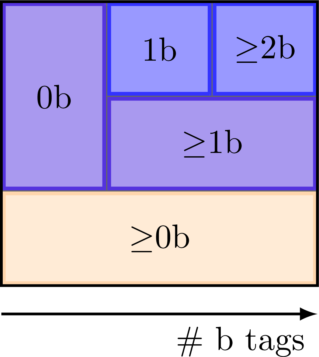
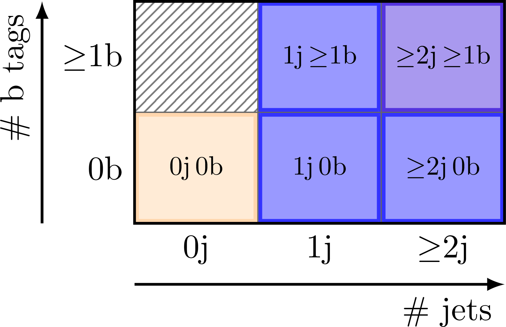
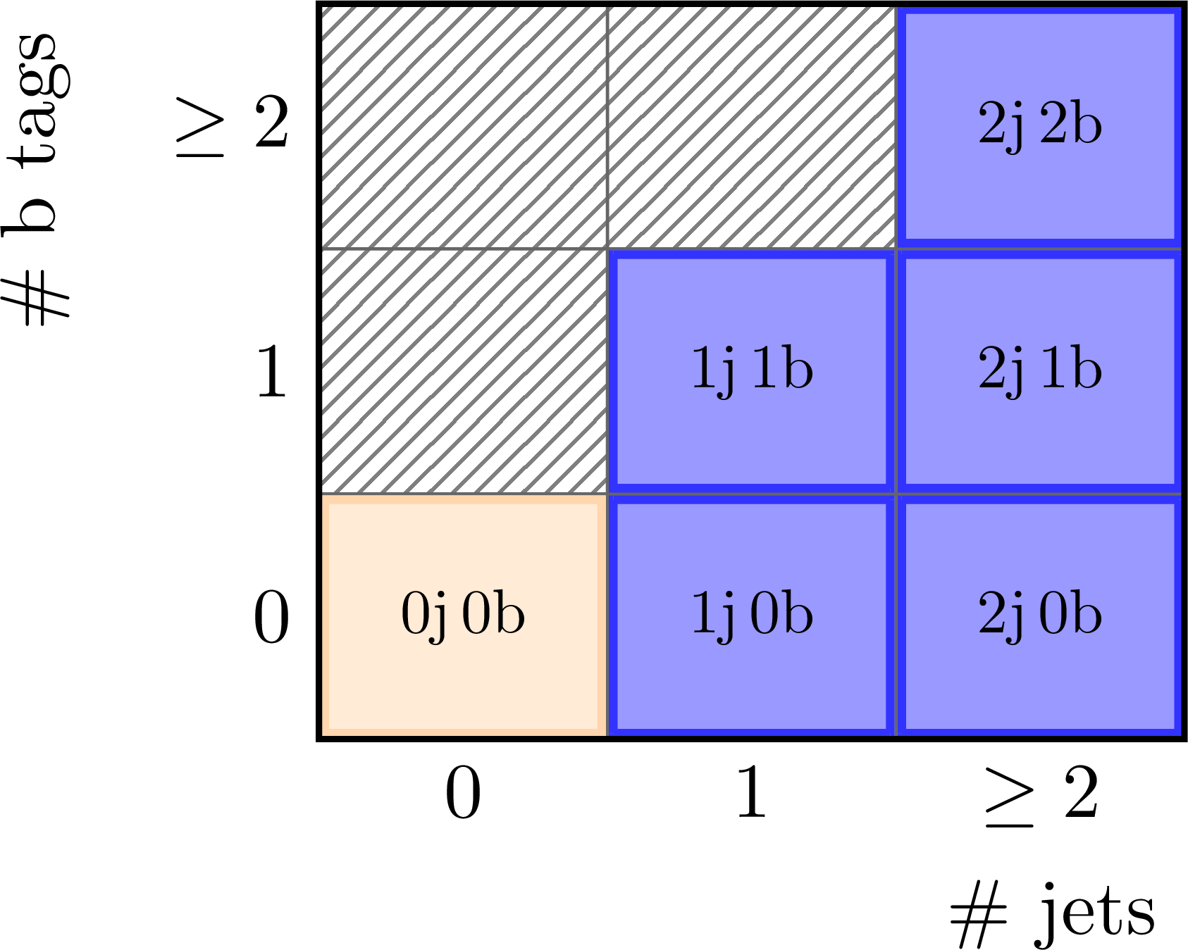
Signal and controls regions in 2D for analyses of proton-proton collision data. Also see the construction of an isolation sideband region, or the ABCD method.

Edit and compile if you like:

% Author: Izaak Neutelings (June, 2017)

\documentclass{article}
\usepackage{amsmath} % for \text
\usepackage{tikz}
\tikzset{>=latex} % for LaTeX arrow head
\usetikzlibrary{patterns} % for hatches area

% colors
\definecolor{mylightred}{RGB}{255,200,200}
\definecolor{mylightblue}{RGB}{172,188,63}
\definecolor{mylightgreen}{RGB}{150,220,150}

% split figures into pages
\usepackage[active,tightpage]{preview}
\PreviewEnvironment{tikzpicture}
\setlength\PreviewBorder{1pt}%

\def\square#1#2#3{
  \draw[thick,#2!80,fill=#2!40,line width=1.1]
    (\ex+#1+\ey) rectangle ++(1-2*\ex,1-2*\ey)
    node[black,midway,scale=0.8] {#3};
}
\def\rectangle#1#2#3#4{
  \draw[thick,#3!80,fill=#3!40,line width=1.1]
    (\ex+#1+\ey) rectangle ++(-2*\ex+#2-2*\ey)
    node[black,midway,scale=1] {#4};
}

\begin{document}



% JET CATEGORIES
\begin{tikzpicture}[scale=1.1,yscale=0.9]
  
  \def\d{0.5}
  \def\ex{0.023}
  \def\ey{0.026}
  
  % GRID
  \foreach \i in {1,2,3}{
    \draw[black!60] (0,\i) -- (4,\i);
    \draw[black!60] (\i,0) -- (\i,3);
  }
  
  % SIGNAL REGIONS
  \rectangle{0,0}{1,3}{orange!40!white}{0j}
  \rectangle{1,1}{1,2}{blue!84!red}{1j}
  \rectangle{2,2}{1,1}{blue}{2j}
  \rectangle{3,2}{1,1}{blue}{$\geq$3j}
  \rectangle{2,1}{2,1}{blue!84!red}{$\geq$2j}
  \rectangle{1,0}{3,1}{blue}{$\geq$1j}
  
  % AXIS
  \draw[thick]
    (0,0) rectangle ++(4,3);
  \draw[->,thick]
    (0,-0.3) --++ (4,0) node[below left] {\# jets};
  
\end{tikzpicture}



% B TAG CATEGORIES
\begin{tikzpicture}[scale=1.1,yscale=0.9]
  
  \def\d{0.5}
  \def\ex{0.0235}
  \def\ey{0.026}
  
  % GRID
  \foreach \i in {1,2,3}{
    \draw[black!60] (0,\i) -- (3,\i);
    \draw[black!60] (\i,0) -- (\i,3);
  }
  
  % SIGNAL REGIONS
  \rectangle{0,0}{3,1}{orange!40!white}{$\geq$0b}
  \rectangle{0,1}{1,2}{blue!84!red}{0b}
  \rectangle{1,1}{2,1}{blue!84!red}{$\geq$1b}
  \rectangle{1,2}{1,1}{blue}{1b}
  \rectangle{2,2}{1,1}{blue}{$\geq$2b}
  
  % AXIS
  \draw[thick]
    (0,0) rectangle ++(3,3);
  \draw[->,thick]
    (0,-0.3) --++ (3,0) node[below left] {\# b tags};
  
\end{tikzpicture}



% SIGNAL REGIONS JETS
\begin{tikzpicture}[scale=1.3,xscale=1,yscale=0.9]
  
  \def\d{0.5}
  \def\ex{0.020}
  \def\ey{0.022}
  
  % FORBIDDEN
  \fill[pattern=north east lines, pattern color=black!50]
    (0,1) rectangle ++(1,1);
  
  % GRID
  \foreach \i in {1,2}{
    \draw[black!60] (0,\i) -- (3,\i);
    \draw[black!60] (\i,0) -- (\i,2);
  }
  
  % SIGNAL REGIONS
  \square{0,0}{orange!40!white}{0j\,0b}
  \square{1,0}{blue}{1j\,0b}
  \square{2,0}{blue}{$\geq$2j\,0b}
  \square{1,1}{blue}{1j\,$\geq$1b}
  \square{2,1}{blue!84!red}{$\geq$2j\,$\geq$1b}
  
  % AXIS
  \draw[thick]
    (0,0) rectangle ++(3,2);
  \draw
    (0+\d,0) node[below] {0j}
    (1+\d,0) node[below] {1j}
    (2+\d,0) node[below] {$\geq$2j};
    %(3,-0.4) node[below left] {\# jets};
  \draw
    (0,0+\d) node[left] {0b}
    (0,1+\d) node[left] {$\geq$1b};
    %(-1.2,2) node[below left,rotate=90] {\# b tags};
  \draw[->,thick]
    (0,-0.55) --++ (3,0) node[below left] {\# jets};
  \draw[->,thick]
    (-0.75,0) --++ (0,2) node[above left,rotate=90] {\# b tags};
    
\end{tikzpicture}



% SIGNAL REGIONS JETS
\begin{tikzpicture}[scale=1.3,yscale=0.85]
  
  \def\d{0.5}
  \def\ex{0.020}
  \def\ey{0.0235}
  
  % FORBIDDEN
  \fill[pattern=north east lines, pattern color=black!50]
    (0,1) -- (1,1) -- (1,2) -- (2,2) -- (2,3) -- (0,3) -- cycle;
  
  % GRID
  \foreach \i in {1,2}{
    \draw[black!60] (0,\i) -- (3,\i);
    \draw[black!60] (\i,0) -- (\i,3);
  }
  
  % SIGNAL REGIONS
  \square{0,0}{orange!40!white}{0j\,0b}
  \square{1,0}{blue}{1j\,0b}
  \square{2,0}{blue}{2j\,0b}
  \square{1,1}{blue}{1j\,1b}
  \square{2,1}{blue}{2j\,1b}
  \square{2,2}{blue}{2j\,2b}
    
  % AXIS
  \draw[thick]
    (0,0) rectangle ++(3,3);
  \draw
    (0+\d,0) node[below] {0}
    (1+\d,0) node[below] {1}
    (2+\d,0) node[below] {$\geq2$}
    (3,-0.46) node[below left] {\# jets};
  \draw
    (0,0+\d) node[left] {0}
    (0,1+\d) node[left] {1}
    (0,2+\d) node[left] {$\geq2$}
    (-1.2,3) node[below left,rotate=90] {\# b tags};
    
\end{tikzpicture}



\end{document}