")


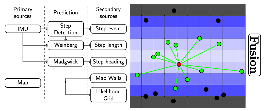
This figure represents a data fusion system used for pedestrian indoor localisation. It is from a scientific paper published in IEEE Sensors 2023 with the following DOI https://doi.org/10.1109/JSEN.2022.3222639.
On the left part, the primary and secondary stages of fusion, that leverage the inertial data (IMU) and the building’s map, are detailed in a bloc scheme. On the right is one of the contribution of this paper: the human motion likelihood representation in the form of a grid. The grid allows to assign a weight to each particle the system uses. Such system is called a Particle Filter.
For usage and reproduction, this figure falls under the IEEE Sensors 2023 copyright. It requires proper citation of the provided paper via its DOI.
\documentclass[tikz,border=10pt]{standalone}
\usetikzlibrary{positioning, calc}
\begin{document}
  \begin{tikzpicture}[
    dot/.style = {circle, minimum size= 8,fill,inner sep=0pt, outer sep=0pt},
    dot/.default = 5pt
  ]
  % Drawing the likelihood grid
  % Horizontal cells count
    \def\lowbound{0}
    \def\highbound{9}

    \begin{scope}[shift={(0,0.5)}, scale=0.7]
      \tikzstyle{cell} = [rectangle, minimum size = 19.5 , fill, color = black]
      \draw [black, step = 1] (\lowbound, 1) grid (\highbound+1, 10);

      \begin{scope}[shift = {(0.5,0.5)}, opacity = 0.7]
        \foreach \x in {\lowbound,1,...,\highbound}{
         \node [cell, black] at  (\x, 9) {};
         \node [cell, black] at  (\x, 1) {};
        } % black cells = walls
        \foreach \x in {\lowbound, 1,..., \highbound}{
         \node [cell, color = blue!100!white] at  (\x, 8) {};
         \node [cell, color = blue!100!white] at  (\x, 2) {};
        } % deep blue cells
        \foreach \x in {\lowbound,1,...,\highbound}{
         \node [cell, color = blue!75!white] at  (\x, 7) {};
         \node [cell, color = blue!75!white] at  (\x, 3) {};
        }
        \foreach \x in {\lowbound,1,...,\highbound}{
         \node [cell, color = blue!30!white] at  (\x, 6){};
         \node [cell, color = blue!30!white] at  (\x, 4){};
        }
        \foreach \x in {\lowbound,1,...,\highbound}{
         \node [cell, color = blue!20!white] at  (\x, 5){};
        }
      \end{scope}
      % Adding particles with random numbers drawn from a python script
      % Yes, LaTeX/Tikz allow to draw random numbers but these come from an experiment
      \begin{scope}
        \coordinate [dot] (a) at (3.9285231, 2.6985591);
        \coordinate [dot] (b) at (1.3611608, 1.9969122);
        \coordinate [dot] (c) at (0.6288356, 3.84908  );
        \coordinate [dot] (e) at (9.6810041, 4.1691515);
        \coordinate [dot] (f) at (7.644834 , 8.55942  );
        \coordinate [dot] (g) at (6.0297038, 7.0389246);
        \coordinate [dot] (h) at (3.2925639, 6.6886047);
        \coordinate [dot] (i) at (1.3797099, 8.5992524);
        \coordinate [dot] (j) at (8.1116873, 2.1354121);
        \coordinate [dot] (k) at (7.7211166, 6.5463598);
        \coordinate [dot] (l) at (6.5935806, 2.6034567);
        \coordinate [dot] (m) at (3.9761724, 6.4383623);
        \coordinate [dot] (n) at (2.4039057, 5.6784096);
        \coordinate [dot] (o) at (4.9582929, 3.4551362);
        \coordinate [dot] (p) at (3.7579452, 1.5857479);
        \coordinate [dot] (q) at (6.2010185, 4.215724 );
        \coordinate [dot] (r) at (2.0341973, 5.4074832);
        \coordinate [dot] (s) at (3.8130486, 9.4286342);
        \coordinate [dot] (t) at (7.518949 , 1.857585 );
        \coordinate [dot] (u) at (2.1995326, 2.236611 );
      \end{scope}

      % circle on top of each coordinate
      \foreach \i in {a,c,e,k,n,r,m,o,q,h,g}
        \draw [green, fill] (\i) circle [radius = 0.15];

      % draw the conenction to the green particles
      \coordinate [dot] (mean) at (4.2424450, 4.7708627);
      \draw [red, fill] (mean) circle [radius = 0.15];
      \draw (mean) edge
        [stroke=black, very thick, green, shorten <=2, shorten >=2] (a);
      \draw (mean) edge
        [stroke, very thick, green, shorten <=2, shorten >=2] (c);
      \draw [stroke, very thick, green, shorten <=2, shorten >=2]
        (mean) -- (e);

        % shorten allows to cut the edge before reaching a node
      \foreach \i in {k,n,r,m,o,q,h,g}
        \draw (mean) edge [very thick, green, shorten <=2, shorten >=2] (\i);

      \begin{scope}[shift={(10.8,5.6)}]
        \node [rotate=-90,
        thick,
        rectangle,
        rounded corners,
        draw,
        text width=,
        minimum height=15,
        align = center](fusion) {\huge\textbf{Fusion}};
      \end{scope}
    \end{scope}

    \begin{scope}[
      shift={(-6.5,7)},
      scale=1, font = {\sffamily},
      every path/.style = {thick},
      every node/.style = {
      thick,
      rectangle,
      rounded corners,
      draw,
      text width = 55,
      minimum height = 12,
      align=center
      },
      empty/.style={color = white, text= black},
      void/.style={fill = white, minimum size = 0}
    ]

      % This is one way to define space between blocs:
      \def\hspacer{0.5} % spacing between columns
      \def\vspacer{1} % spacing between lines

      %%%%%%% Acquisition
      \node[empty] (input) {Primary sources};
      \node[below of = input] (imu) {IMU};
      \node[below of = imu, below = 2*\vspacer] (map) {Map};
      \coordinate [below of = map] (dots);

      %%%%%%%% Prediction
      \node[right of = input, right = \hspacer, empty] (prediction) {Prediction};
      \node[below of = prediction] (detect) {Step Detection};
      \node[below of = detect] (weinberg) {Weinberg};
      \node[below of = weinberg] (madgwick) {Madgwick};

      %%%%%%%%% Output
      \node[right of = prediction, right = \hspacer, empty] (output)
       {Secondary sources};
      \node[below of = output] (events) {Step event};
      \node[below of = events] (lengths) {Step length};
      \node[below of = lengths] (angles) {Step heading};

      \node[below of = angles] (walls) {Map Walls};
      \node[below of = walls] (grid) {Likelihood Grid};

      %% Links
      \draw [->] (imu)--(detect);
      \draw [->] (imu)|-(weinberg);
      %
      \draw [->] (imu)|-(madgwick);
      %
      \draw [->] (detect)--(events);
      \draw [->] (weinberg)--(lengths);
      \draw [->] (detect)--(weinberg);
      %
      \draw [->] (madgwick)--(angles);
      %
      \draw [->] (map.east)  -| ($(map)!0.5!(walls)$) coordinate |-(walls);
      \draw [->] (map)       -| ($(map)!0.5!(walls)$)            |-(grid);
      %

      % Draw columns sperators

      \draw [dashed] ($(input.north)     !0.5!(prediction.north)$)
        --($(input)     !0.5!(prediction)+(dots.south)$);
      \draw [dashed] ($(prediction.north)!0.5!(output.north)$)
        --($(prediction)!0.5!(output)    +(dots.south)$);
    \end{scope}
  \end{tikzpicture}
\end{document}