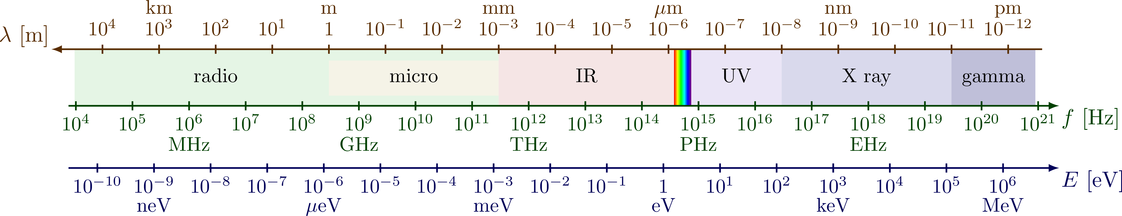
Electromagnetic spectrum

Edit and compile if you like:

1
2
3
4
5
6
7
8
9
10
11
12
13
14
15
16
17
18
19
20
21
22
23
24
25
26
27
28
29
30
31
32
33
34
35
36
37
38
39
40
41
% Author: Izaak Neutelings (May 2020)
\documentclass[border=3pt,tikz]{standalone}
\tikzset{>=latex} % for LaTeX arrow head
\usepackage{ifthen}
\usepackage{xcolor}
\usepackage{physics}
\usepackage{siunitx}
\colorlet{wavecol}{orange!35!black}
\colorlet{freqcol}{green!25!black}
\colorlet{enercol}{blue!35!black}
\pgfdeclareverticalshading{rainbow}{100bp}{
  color(0bp)=(red); color(25bp)=(red); color(35bp)=(yellow);
  color(45bp)=(green); color(55bp)=(cyan); color(65bp)=(blue);
  color(75bp)=(violet); color(100bp)=(violet)
}
\begin{document}
% ELECTROMAGNETIC SPECTRUM
\begin{tikzpicture}[xscale=1]
  \def\h{1}
  \def\radio{-4}
  \def\micro{0}
  \def\IR{3}
  \def\red{6.10}  % log(700e-9) = -6.15490196
  \def\blue{6.40} % log(400e-9) = -6.39794001
  \def\UV{6.40}
  \def\Xray{8}
  \def\gamm{11}
  \def\last{12}
  \def\radiof{-5}
  \def\dx{0.6}
  \def\yE{-1.1*\h}
  
  \def\tick#1#2#3{\draw[thick,#2] (#1+.08) --++ (0,-.16) node[below=-2pt,scale=1] {\strut #3};}
  \def\ticka#1#2#3{\draw[thick,#2] (#1+.08) --++ (0,-.16) node[above=2pt,scale=1] {\strut #3};}
  
  % MIDDLE
 
 
הההההההההההההההההההההההההההההההההההההההההההההההההההההההההההההההההההההההההההההההההההההההההההההההההההההההההההההההההההההההההההההההההההההההההההההההההההההההההההההההההההההההההההההההההההההההההההההההההההההההההההההההההההההההההההההההההההההההההההההההההההההההההההההההה
XXXXXXXXXXXXXXXXXXXXXXXXXXXXXXXXXXXXXXXXXXXXXXXXXXXXXXXXXXXXXXXXXXXXXXXXXXXXXXXXXXXXXXXXXXXXXXXXXXXXXXXXXXXXXXXXXXXXXXXXXXXXXXXXXXXXXXXXXXXXXXXXXXXXXXXXXXXXXXXXXXXXXXXXXXXXXXXXXXXXXXXXXXXXXXXXXXXXXXXXXXXXXXXXXXXXXXXXXXXXXXXXXXXXXXXXXXXXXXXXXXXXXXXXXXXXXXXX