Pressure variation over altitude

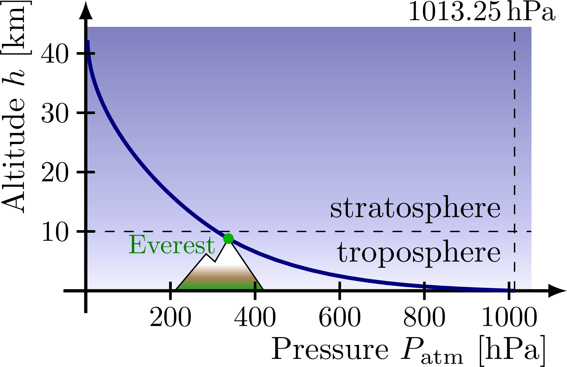
The atmospheric pressure variation as a function of altitude.

Air pressure over altitude:

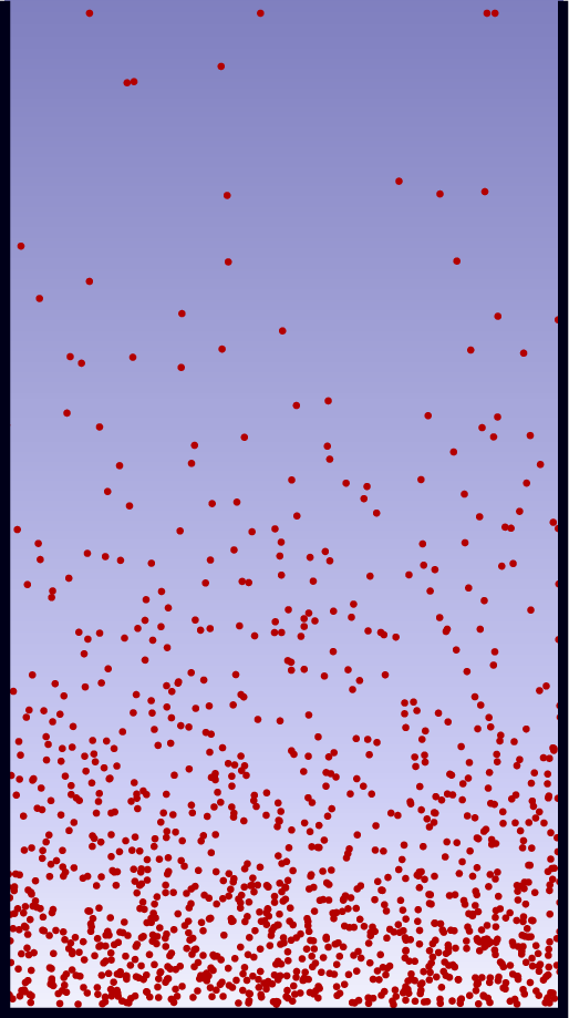
Air density over altitude:

Edit and compile if you like:

1
2
3
4
5
6
7
8
9
10
11
12
13
14
15
16
17
18
19
20
21
22
23
24
25
26
27
28
29
30
31
32
33
34
35
36
37
38
39
40
41
% Author: Izaak Neutelings (November 2020)
\documentclass[border=3pt,tikz]{standalone}
\usepackage{siunitx}
%\usepackage{physics}
\usepackage{tikz}
%\usepackage[outline]{contour} % glow around text
\usetikzlibrary{patterns,decorations.pathmorphing}
\usetikzlibrary{arrows.meta}
\tikzset{>=latex}
%\contourlength{1.1pt}
\colorlet{mydarkblue}{blue!50!black}
\colorlet{myred}{red!65!black}
\tikzstyle{force}=[->,myred,very thick,line cap=round]
\tikzstyle{vvec}=[->,very thick,vcol,line cap=round]
\def\tick#1#2{\draw[thick] (#1)++(#2:0.1) --++ (#2-180:0.2)}
\begin{document}
% ATMOSPHERIC PRESSURE vs. ALTITUDE
\begin{tikzpicture}
  \def\xmax{4.9}
  \def\ymax{2.9}
  \def\Nx{5}
  \def\Ny{4}
  \coordinate (M) at (0.95*\xmax*3.37/2/\Nx,0.9*\ymax*0.88/\Ny); % mount Everest
  \coordinate (S) at (0.95*\xmax*10.13/2/\Nx,0); % sea level
  
  % SKY + MOUNTAIN
  \fill[top color=blue!80!black!20,bottom color=blue!80!black!5]
    (0,0) rectangle (\xmax,0.9/\Ny*\ymax);
  \fill[top color=blue!50!black!50,bottom color=blue!80!black!20]
    (0,0.9/\Ny*\ymax) rectangle (\xmax,\ymax);
  \begin{scope}
    \clip (0.2*\xmax,0) --++ (0.07*\xmax,0.14*\ymax) --++ (0.02*\xmax,-0.03*\ymax) -- (M) -- (0.4*\xmax,0);
    \fill[white] (0.1*\xmax,0) rectangle (0.4*\xmax,0.5*\ymax);
    \fill[top color=white,bottom color=green!60!black!90,middle color=brown!80!black!80]
      (0.1*\xmax,0) rectangle (0.4*\xmax,0.1*\ymax);
  \end{scope}
  \draw[thin] (0.2*\xmax,0) --++ (0.07*\xmax,0.14*\ymax) --++ (0.02*\xmax,-0.03*\ymax) -- (M) -- (0.4*\xmax,0);
 
 
הההההההההההההההההההההההההההההההההההההההההההההההההההההההההההההההההההההההההההההההההההההההההההההההההההההההההההההההההההההההההההההההההההההההההההההההההההההההההההההההההההההההההההההההההההההההההההההההההההההההההההההההההההההההההההההההההההההההההההההההההההההההההההההההה
XXXXXXXXXXXXXXXXXXXXXXXXXXXXXXXXXXXXXXXXXXXXXXXXXXXXXXXXXXXXXXXXXXXXXXXXXXXXXXXXXXXXXXXXXXXXXXXXXXXXXXXXXXXXXXXXXXXXXXXXXXXXXXXXXXXXXXXXXXXXXXXXXXXXXXXXXXXXXXXXXXXXXXXXXXXXXXXXXXXXXXXXXXXXXXXXXXXXXXXXXXXXXXXXXXXXXXXXXXXXXXXXXXXXXXXXXXXXXXXXXXXXXXXXXXXXXXXX