B tagging jets

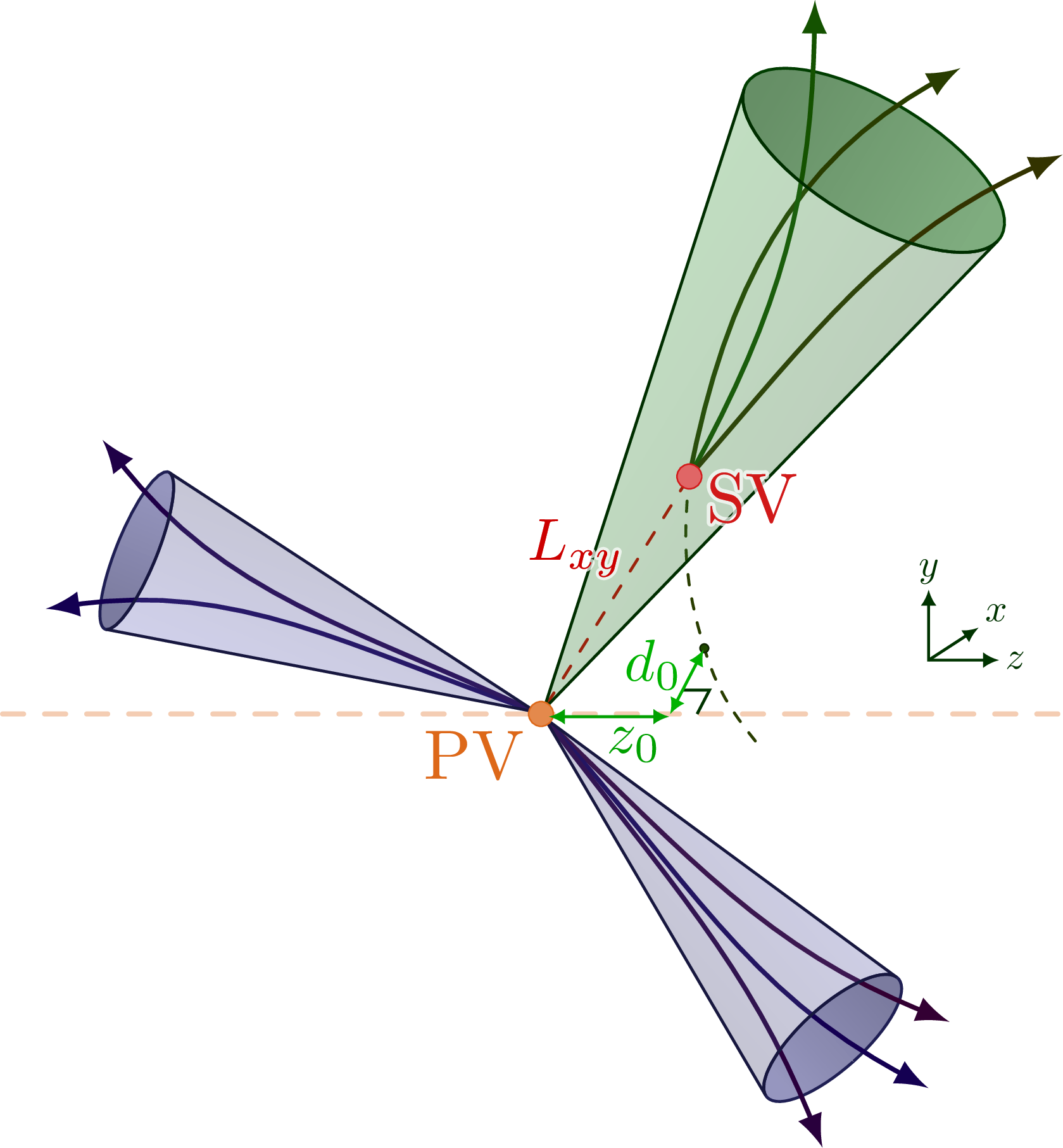
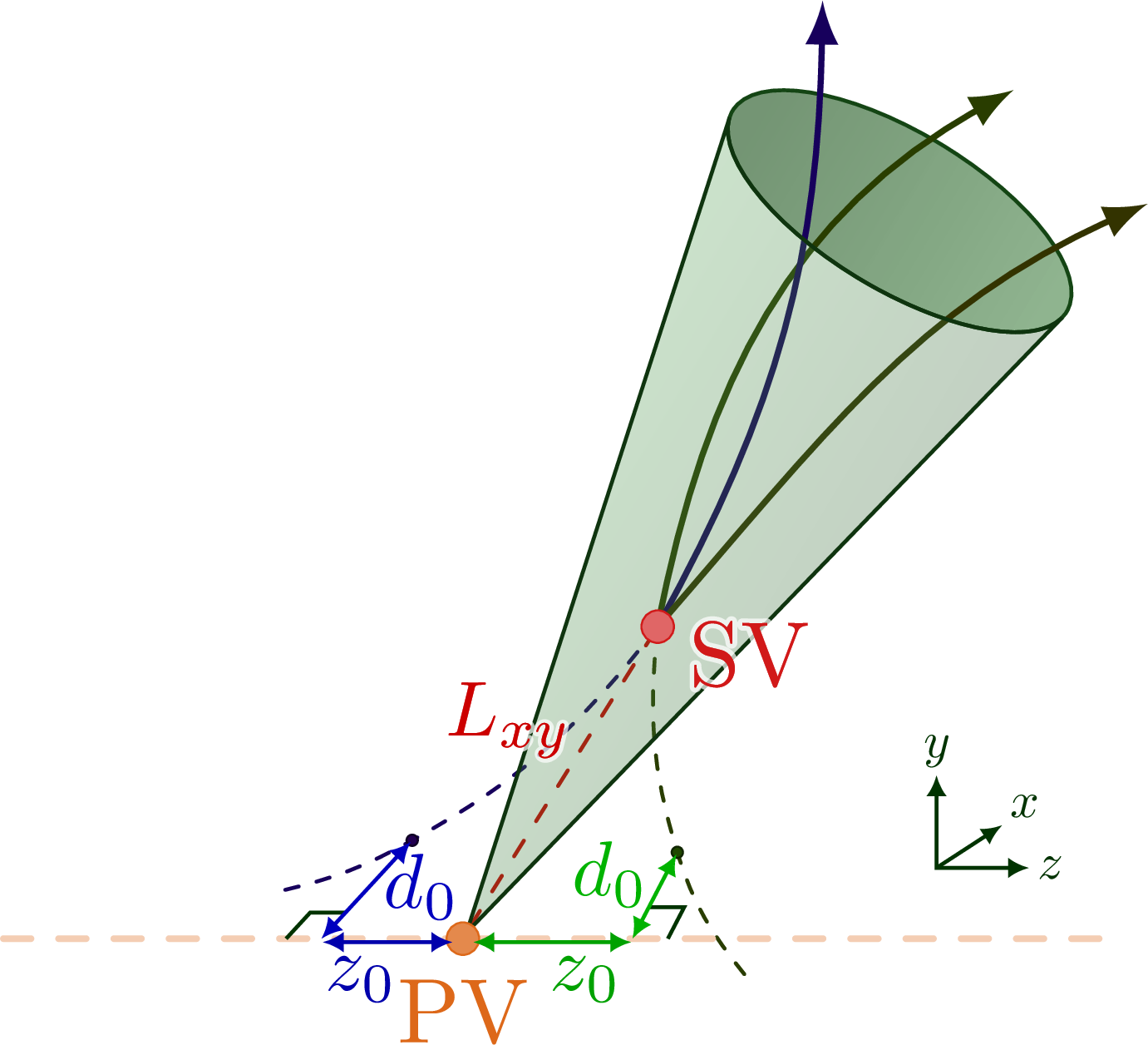
Characteristics of a jet initiated by a bottom quark: secondary vertex, as well as a longitudinal (z₀) and transverse impact parameter (d₀) of individual tracks from their point of closest approach to the primary vertex.
For more related figures, please see the “jet” tag or the Particle Physics category. The cones are constructed with the tangent methods presented here.

Edit and compile if you like:

1
2
3
4
5
6
7
8
9
10
11
12
13
14
15
16
17
18
19
20
21
22
23
24
25
26
27
28
29
30
31
32
33
34
35
36
37
38
39
40
41
% Author: Izaak Neutelings (July 2021)
% Description: B tagging of a jet
% Inspiration: Nazar Bartosik, https://commons.wikimedia.org/wiki/File:B-tagging_diagram.png
%  https://indico.cern.ch/event/687697/contributions/2825792/attachments/1579225/2494980/bjet_tagging_via_trackIP.pdf
%  B tagging algorithm at ATLAS: https://arxiv.org/abs/1711.08811
%  B tagging algorithm at CMS: https://arxiv.org/abs/1712.07158
\documentclass[border=3pt,tikz]{standalone}
\usepackage{amsmath}
%\usepackage{physics}
\usepackage{xcolor}
\usepackage[outline]{contour} % glow around text
\usetikzlibrary{calc}
\usetikzlibrary{math} % for \tikzmath
\usetikzlibrary{arrows.meta}
\usetikzlibrary{decorations.pathreplacing} % for curly braces
\contourlength{0.5pt}
\tikzset{>=latex} % for LaTeX arrow head
\colorlet{myred}{red!80!black}
\colorlet{myblue}{blue!75!black}
\colorlet{mydarkblue}{blue!40!black}
\colorlet{mygreen}{green!50!black}
\colorlet{mylightgreen}{green!70!black}
\colorlet{mydarkgreen}{green!20!black}
\colorlet{myorange}{orange!80!red!85!black}
\tikzstyle{cone}=[thin,blue!50!black,fill=blue!50!black!30] %,fill opacity=0.8
\tikzstyle{track}=[->,line width=0.65,blue!40!black]
\tikzstyle{beam}=[myorange!30,dashed,line width=0.7,line cap=round]
\tikzstyle{conebase}=[cone,fill=blue!50!black!50] %,fill opacity=0.8
\tikzstyle{mydashed}=[dash pattern=on 2pt off 2.5pt,line cap=round]
\tikzstyle{myshortdashed}=[dash pattern=on 1.5pt off 2pt,line cap=round]
\tikzstyle{measure}=[{Latex[length=2.2,width=2.2]}-{Latex[length=2.2,width=2.2]}]
\newcommand\jetcone[6][blue]{{
  \pgfmathanglebetweenpoints{\pgfpointanchor{#2}{center}}{\pgfpointanchor{#3}{center}}
  \edef\ang{#4/2}
  \edef\e{#5}
  \edef\vang{\pgfmathresult} % angle of vector OV
  \tikzmath{
    coordinate \C;
    \C = (#2)-(#3);
 
 
הההההההההההההההההההההההההההההההההההההההההההההההההההההההההההההההההההההההההההההההההההההההההההההההההההההההההההההההההההההההההההההההההההההההההההההההההההההההההההההההההההההההההההההההההההההההההההההההההההההההההההההההההההההההההההההההההההההההההההההההההההההההההההההההה
XXXXXXXXXXXXXXXXXXXXXXXXXXXXXXXXXXXXXXXXXXXXXXXXXXXXXXXXXXXXXXXXXXXXXXXXXXXXXXXXXXXXXXXXXXXXXXXXXXXXXXXXXXXXXXXXXXXXXXXXXXXXXXXXXXXXXXXXXXXXXXXXXXXXXXXXXXXXXXXXXXXXXXXXXXXXXXXXXXXXXXXXXXXXXXXXXXXXXXXXXXXXXXXXXXXXXXXXXXXXXXXXXXXXXXXXXXXXXXXXXXXXXXXXXXXXXXXX

Click to download: jet_btag.tex • jet_btag.pdf
Open in Overleaf: jet_btag.tex