Nonconvex Solid

Edit and compile if you like:

\documentclass{article}
%
% File name: nonconvex-solid.tex
% Description: 
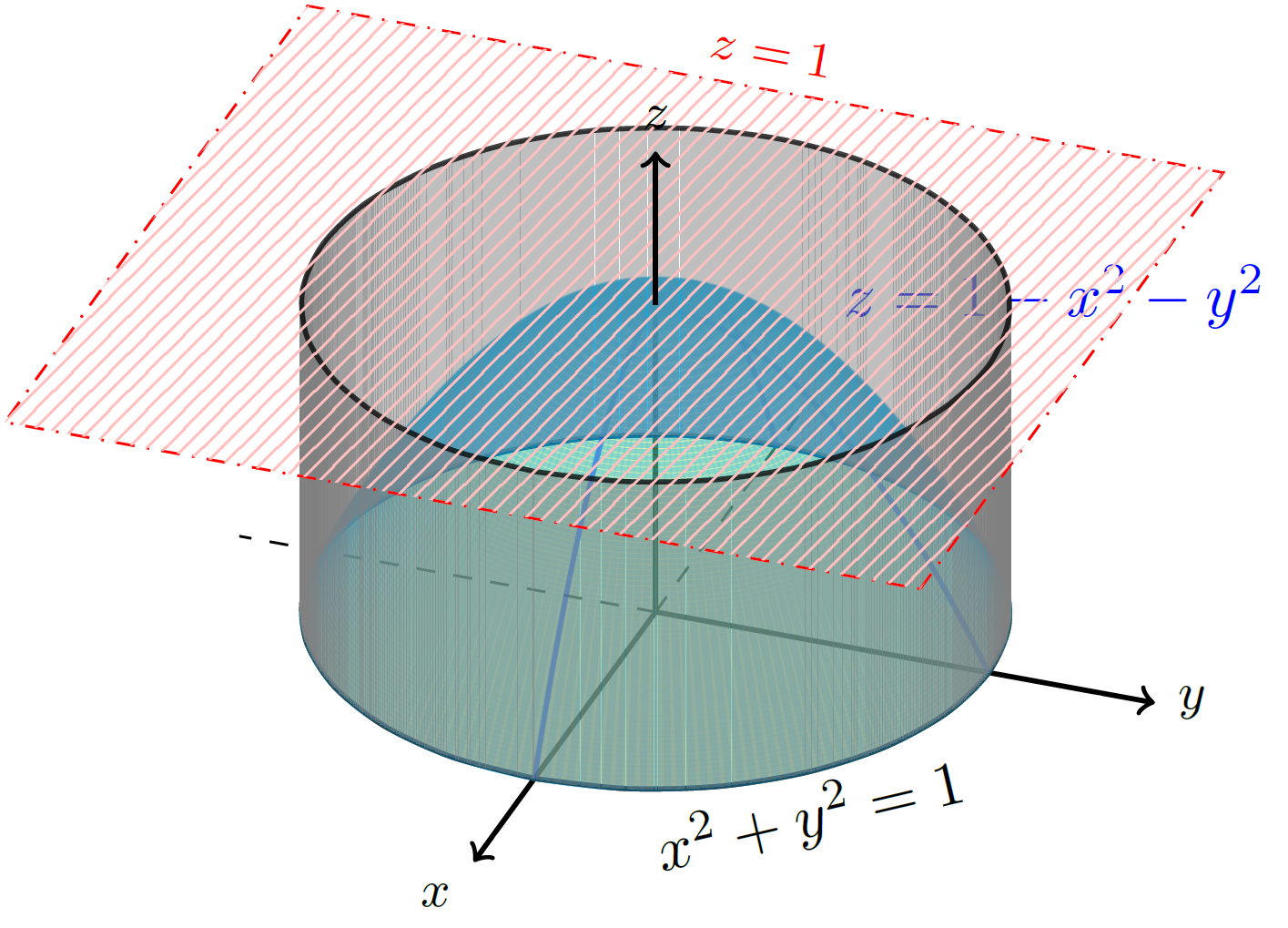
% The solid bounded by the graphs of the surfaces:
% z = 1 - x^{2} - y^{2}
% z = 1
% x^2 + y^2 = 1
% is generated. Also, the region x^2 + y^2 \leq 1
% is shown.
% 
% Date of creation: April, 23rd, 2022.
% Date of last modification: April, 23rd, 2022.
% Author: Efraín Soto Apolinar.
% https://www.aprendematematicas.org.mx/author/efrain-soto-apolinar/instructing-courses/
% Terms of use:
% According to TikZ.net
% https://creativecommons.org/licenses/by-nc-sa/4.0/
% 
\usepackage{tikz}
\usetikzlibrary{patterns}
\usepackage{tikz-3dplot}
\usepackage[active,tightpage]{preview}
\PreviewEnvironment{tikzpicture}
\setlength\PreviewBorder{1pt}
%
\begin{document}
	%
	\tdplotsetmaincoords{60}{110}
	\begin{tikzpicture}[tdplot_main_coords,scale=2.0]
		\pgfmathsetmacro{\tini}{0.5*pi}
		\pgfmathsetmacro{\tfin}{1.85*pi}
		\pgfmathsetmacro{\tend}{2.5*pi}
		\pgfmathsetmacro{\final}{2.0*pi}
		\coordinate (A) at (1.25,1.25,1);
		\coordinate (B) at (-1.25,1.25,1);
		\coordinate (C) at (-1.25,-1.5,1);
		\coordinate (D) at (1.25,-1.5,1);
		% Node indicating the equation of the circumference
		\draw[white] (1.35,0,0) -- (0,1.35,0) node [black,below,midway,sloped] {$x^2 + y^2 = 1$};
		%%% Coordinate axis
		\draw[thick,->] (0,0,0) -- (1.5,0,0) node [below left] {\footnotesize$x$};
		\draw[dashed] (0,0,0) -- (-1.25,0,0);
		\draw[thick,->] (0,0,0) -- (0,1.5,0) node [right] {\footnotesize$y$};
		\draw[dashed] (0,0,0) -- (0,-1.25,0);
		\draw[thick] (0,0,0) -- (0,0,1.0);
		% The region of integration
		\fill[yellow,opacity=0.35] plot[domain=0:6.2832,smooth,variable=\t] ({cos(\t r)},{sin(\t r)},{0.0});
		\draw[gray,thick] plot[domain=0:6.2832,smooth,variable=\t] ({cos(\t r)},{sin(\t r)},{0.0});
		% Circunference bounding the surface (for z = 0)
		\draw[black,thick,opacity=0.75] plot[domain=0:6.2832,smooth,variable=\t] ({cos(\t r)},{sin(\t r)},{0.0}); 
		% The curves slicing the surface
		\draw[blue,thick,opacity=0.5] plot[domain=-1:1,smooth,variable=\t] ({\t},0,{1.0 - \t*\t}); 
		\draw[blue,thick,opacity=0.5] plot[domain=-1:1,smooth,variable=\t] (0,{\t},{1.0 - \t*\t}); 
		\foreach \angulo in {0,2,...,358}{
			\draw[cyan,very thick,rotate around z=\angulo,opacity=0.15] plot[domain=0:1,smooth,variable=\t] ({0},{\t},{1.0 - \t*\t});
		}
		% El paraboloid (for z = constant)
		\foreach \altura in {0.0125,0.025,...,1.0}{
			\pgfmathparse{sqrt(\altura)}
			\pgfmathsetmacro{\radio}{\pgfmathresult}
			\draw[cyan,thick,opacity=0.35] plot[domain=\tini:\tfin,smooth,variable=\t] ({\radio*cos(\t r)},{\radio*sin(\t r)},{1.0 - \altura}); 
		}
		% First part of the z axis
		\draw[thick,->] (0,0,1.0) -- (0,0,1.5) node [above] {\footnotesize$z$};	
		\foreach \altura in {0.0125,0.025,...,1.0}{
			\pgfmathparse{sqrt(\altura)}
			\pgfmathsetmacro{\radio}{\pgfmathresult}
			\draw[cyan,thick,opacity=0.35] plot[domain=\tfin:\tend,smooth,variable=\t] ({\radio*cos(\t r)},{\radio*sin(\t r)},{1.0 - \altura}); 
		}
		%
		\node[blue,right] at (0,0.5,1.125) {$z = 1 - x^2 - y^2$};
		% The outer cylinder
		\foreach \angulo in {0,0.01,...,\final}{
			\pgfmathparse{cos(\angulo r)}
			\pgfmathsetmacro{\px}{\pgfmathresult}
			\pgfmathparse{sin(\angulo r)}
			\pgfmathsetmacro{\py}{\pgfmathresult}
			\draw[gray,opacity=0.5] (\px,\py,0) -- (\px,\py,1.0);
		}
		% The circumference at z = 1
		\draw[black,thick,opacity=0.75] plot[domain=0:6.2832,smooth,variable=\t] ({cos(\t r)},{sin(\t r)},{1.0}); 
		% The plane z = 1.
		\draw[white] (C) -- (B) node[red,above,sloped,midway]{\footnotesize$z = 1$};
		\draw[red,dash dot] (A) -- (B) -- (C)	 -- (D) -- (A);
		\fill[pattern color=pink,pattern=north east lines] (A) -- (B) -- (C)	 -- (D) -- (A);
		%
		\draw[thick,->] (0,0,1.0) -- (0,0,1.5) node [above] {\footnotesize$z$};
	\end{tikzpicture}
\end{document}