")


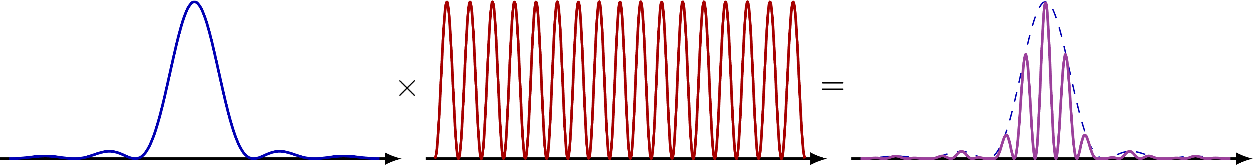
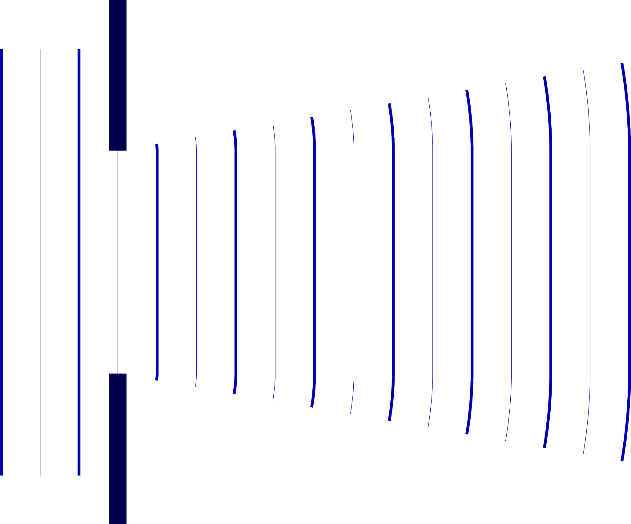
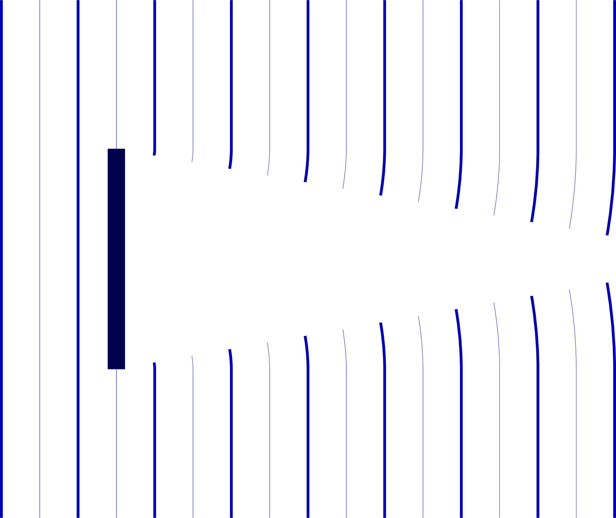
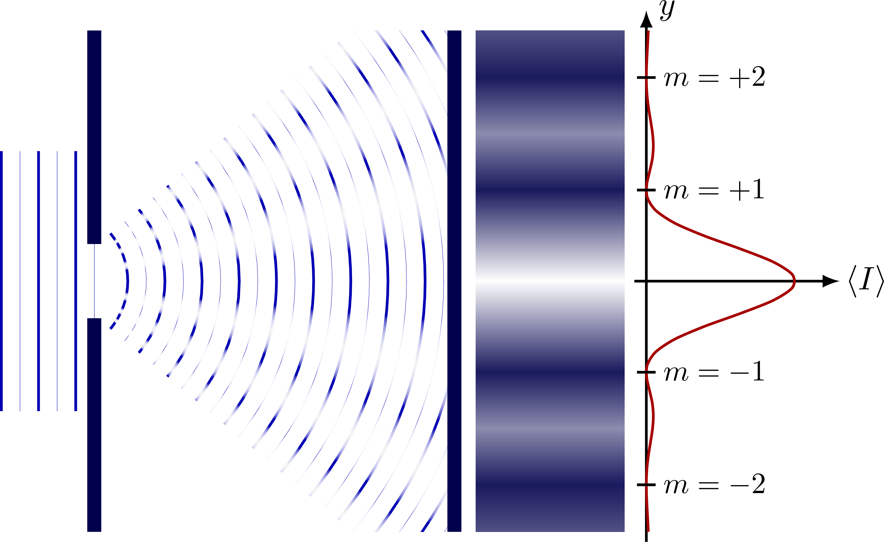
Diffraction of light through a small slit, around an obstacle, around a corner, as well as the interference pattern (Fraunhofer equation) and dispersion due to diffraction. For more related figures, please see the Optics category.


% Author: Izaak Neutelings (June 2020)
% Inspiration:
% https://courses.physics.ucsd.edu/2011/Summer/session1/physics2c/diffraction.pdf
% https://tex.stackexchange.com/questions/201830/periodic-shading-in-tikz
\documentclass[border=3pt,tikz]{standalone}
\usepackage[outline]{contour} % glow around text
\usepackage{physics}
\usepackage{xcolor}
\usepackage{etoolbox} %ifthen
\usetikzlibrary{calc}
\usetikzlibrary{arrows,arrows.meta}
\usetikzlibrary{decorations.markings}
\usetikzlibrary{angles,quotes} % for pic (angle labels)
\usetikzlibrary{fadings}
\tikzset{>=latex} % for LaTeX arrow head
\contourlength{1.6pt}
\colorlet{wall}{blue!30!black}
\colorlet{myblue}{blue!70!black}
\colorlet{myred}{red!65!black}
\colorlet{mypurple}{red!50!blue!95!black!75}
\colorlet{myshadow}{blue!30!black!90}
\colorlet{mydarkred}{red!50!black}
\colorlet{mylightgreen}{green!60!black!70}
\colorlet{mygreen}{green!60!black}
\colorlet{myredgrey}{red!50!black!80}
\tikzstyle{wave}=[myblue,thick]
\tikzstyle{mydashed}=[black!70,dashed,thin]
\tikzstyle{mymeas}=[{Latex[length=3,width=2]}-{Latex[length=3,width=2]},thin]
\tikzstyle{mysmallarr}=[-{Latex[length=3,width=2]}]
\tikzset{
declare function={
int_arg(\y,\lam,\a,\L) = \a*\y/sqrt(\L*\L+\y*\y)/\lam; %sin(\x);
int_one(\y,\lam,\a,\L) = (sin(180*int_arg(\y,\lam,\a,\L))/(pi*int_arg(\y,\lam,\a,\L)))^2;
int_two(\y,\lam,\a,\L) = cos(180*int_arg(\y,\lam,\a,\L))^2;
int_arg_ang(\t,\lam,\a) = \a*sin(\t)/\lam;
int_one_ang(\t,\lam,\a) = (sin(180*int_arg_ang(\t,\lam,\a))/(pi*int_arg_ang(\t,\lam,\a)))^2;
int_two_ang(\t,\lam,\a) = cos(180*int_arg_ang(\t,\lam,\a))^2;
}
}
\newcommand\rightAngle[4]{
\pgfmathanglebetweenpoints{\pgfpointanchor{#2}{center}}{\pgfpointanchor{#3}{center}}
\coordinate (tmpRA) at ($(#2)+(\pgfmathresult+45:#4)$);
\draw[white,line width=0.6] ($(#2)!(tmpRA)!(#1)$) -- (tmpRA) -- ($(#2)!(tmpRA)!(#3)$);
\draw[mydarkred] ($(#2)!(tmpRA)!(#1)$) -- (tmpRA) -- ($(#2)!(tmpRA)!(#3)$);
}
\newcommand\lineend[2]{
\def\w{0.1} \def\c{30}
\draw[mygreen] (#1)++(#2:\w) to[out=#2-180-\c,in=#2+\c] (#1)
to[out=#2+\c-180,in=#2-\c]++ (#2-180:\w);
}
\def\tick#1#2{\draw[thick] (#1) ++ (#2:0.1) --++ (#2-180:0.2)}
\begin{document}
%% TWO SPLIT: interference x diffraction
%\begin{tikzpicture}
% \def\A{3.5}
% \def\d{3.4} % slit distance
% \def\a{0.9} % slit size
% \def\lambd{0.2} % wavelength
% \def\k{15} % x -> theta
% \def\xmax{4.6}
% \def\ymax{\A}
% \def\N{4}
% \def\D{2.3*\xmax}
% \def\L{4.0}
% \def\nsamples{80}
%
% \draw[->,thick,black] (-1.05*\xmax,0) -- (1.1*\xmax,0) node[below] {$\theta$};
% \draw[->,thick,black] (0,-0.1*\A) -- (0,1.12*\A);
% \draw[wave,variable=\t,samples=\nsamples,smooth,domain=-\xmax:\xmax]
% plot(\t,{\A*int_one_ang(\k*\t,\lambd,\a)});
%
% \foreach \i [evaluate={\t=asin(\i*\lambd/\a)/\k;}] in {1,...,\N}{
% \tick{-\t,0}{90} node[below=-1,scale=0.7] {$m=-\i$};
% \tick{\t,0}{90} node[below=-1,scale=0.7] {$m=+\i$};
% }
%
%\end{tikzpicture}
% TWO SLIT: interference x diffraction
\begin{tikzpicture}
\message{Two slits^^J}
\def\A{1.7}
\def\d{3.4} % slit distance
\def\a{1.2} % slit size
\def\lambd{0.2} % wavelength
\def\k{15} % x -> theta
\def\xmax{2}
\def\D{2.3*\xmax}
\def\L{4.0}
\def\nsamples{80}
% WAVE 1
\draw[->,thick,black]
(-1.05*\xmax,0) -- (1.12*\xmax,0);
\draw[wave,variable=\t,samples=\nsamples,smooth,domain=-\xmax:\xmax]
plot(\t,{\A*int_one_ang(\k*\t,\lambd,\a)});
\node at (\D/2,0.45*\A) {$\times$};
% WAVE 2
\begin{scope}[shift={(\D,0)}]
\draw[->,thick,black]
(-1.05*\xmax,0) -- (1.12*\xmax,0);
\draw[wave,myred,variable=\t,samples=3*\nsamples,smooth,domain=-\xmax:\xmax]
plot(\t,{\A*int_two_ang(\k*\t,\lambd,\d)});
\node at (\D/2,0.45*\A) {$=$};
\end{scope}
% WAVE 3
\begin{scope}[shift={(2*\D,0)}]
\draw[->,thick,black]
(-1.05*\xmax,0) -- (1.12*\xmax,0);
\draw[wave,dashed,thin,variable=\t,samples=\nsamples,smooth,domain=-\xmax:\xmax]
plot(\t,{\A*int_one_ang(\k*\t,\lambd,\a)});
\draw[wave,mypurple,variable=\t,samples=2*\nsamples,smooth,domain=-\xmax:\xmax]
plot(\t,{\A*int_one_ang(\k*\t,\lambd,\a)*int_two_ang(\k*\t,\lambd,\d)});
\end{scope}
\end{tikzpicture}
% DIFFRACTION - large slit - circular
\def\H{5.4} % total wall height
\def\h{4.4} % plane wave height
\def\t{0.18} % wall thickness
\def\a{2.3} % slit size
\def\lambd{0.4} % wavelength
\def\N{14} % number of waves
\def\dN{30} % number shift
\def\ang{6} % angle of diffraction
\begin{tikzpicture}
\message{Diffraction, circular^^J}
\def\lambd{0.4} % wavelength
% WAVES
\foreach \i [evaluate={\r=0.9*\i*\lambd;\R=(\i+\dN)*\lambd;}] in {1,...,\N}{
\ifodd\i
\draw[myblue,line width=0.8] (\r,{\R*sin(\ang)}) arc (\ang:-\ang:\R);
\else
\ifnumless{\i}{\N}{
\draw[myblue!80,line width=0.1] (\r,{\R*sin(\ang)}) arc (\ang:-\ang:\R);
}{}
\fi
}
\foreach \i [evaluate={\xp=-2*(\i-0.5)*\lambd; \xm=-2*(\i-1)*\lambd;}] in {1,...,2}{
\draw[myblue,line width=0.8] (\xp,-\h/2) -- (\xp,\h/2);
\draw[myblue,line width=0.1] (\xm,-\h/2) -- (\xm,\h/2);
}
% WALL
\fill[wall]
(\t/2,\a/2) rectangle (-\t/2,\H/2)
(\t/2,-\a/2) rectangle (-\t/2,-\H/2);
\end{tikzpicture}
% DIFFRACTION - large slit - straight
\def\ang{10} % angle of diffraction
\begin{tikzpicture}
\message{Diffraction, straight^^J}
% WAVES
\foreach \i [evaluate={\r=\i*\lambd;}] in {1,...,\N}{
\ifodd\i
\draw[myblue,line width=0.8] (\r,{\a/2+\r*sin(\ang)}) arc(\ang:0:\r) --++ (0,-\a) arc(0:-\ang:\r);
\else
\ifnumless{\i}{\N}{
\draw[myblue,line width=0.1] (\r,{\a/2+\r*sin(\ang)}) arc(\ang:0:\r) --++ (0,-\a) arc(0:-\ang:\r);
}{}
\fi
}
\foreach \i [evaluate={\xp=-2*(\i-0.5)*\lambd; \xm=-2*(\i-1)*\lambd;}] in {1,...,2}{
\draw[myblue,line width=0.8] (\xp,-\h/2) -- (\xp,\h/2);
\draw[myblue,line width=0.1] (\xm,-\h/2) -- (\xm,\h/2);
}
% WALL
\fill[wall]
(\t/2,\a/2) rectangle (-\t/2,\H/2)
(\t/2,-\a/2) rectangle (-\t/2,-\H/2);
\end{tikzpicture}
% DIFFRACTION - obstacle - straight
\begin{tikzpicture}
\message{Diffraction, obstacle^^J}
% WAVES
\foreach \i [evaluate={\r=\i*\lambd;}] in {1,...,\N}{
\ifodd\i
\draw[myblue,line width=0.8]
(\r,\H/2) -- (\r,0.5*\a) arc (0:-\ang:\r)
(\r,-\H/2) -- (\r,-0.5*\a) arc (0:\ang:\r);
\else
\ifnumless{\i}{\N}{
\draw[myblue!80,line width=0.1]
(\r,\H/2) -- (\r,0.5*\a) arc (0:-\ang:\r)
(\r,-\H/2) -- (\r,-0.5*\a) arc (0:\ang:\r);
}{}
\fi
}
\foreach \i [evaluate={\xp=-2*(\i-0.5)*\lambd; \xm=-2*(\i-1)*\lambd;}] in {1,...,2}{
\draw[myblue,line width=0.8] (\xp,-\H/2) -- (\xp,\H/2);
\draw[myblue,line width=0.1] (\xm,-\H/2) -- (\xm,\H/2);
}
% WALL
\fill[wall] (-\t/2,-\a/2) rectangle (\t/2,\a/2);
\end{tikzpicture}
% DIFFRACTION - small slit
\begin{tikzpicture}
\message{Diffraction, small slit^^J}
\def\H{5.5} % total wall height
\def\h{4.0} % plane wave height
\def\t{0.18} % wall thickness
\def\a{0.68} % slit distance
\def\N{7} % number of waves
\def\lambd{0.4} % wavelength
\def\ang{40}
% WAVES
\foreach \i [evaluate={\Rp=2*\i*\lambd; \Rm=2*(\i+0.5)*\lambd;}] in {1,...,\N}{
\draw[myblue,line width=0.8] (-0.9*\lambd,0)++(\ang:\Rp) arc (\ang:-\ang:\Rp);
\ifnumless{\i}{\N}{
\draw[myblue!80,line width=0.1] (-0.9*\lambd,0)++(\ang:\Rm) arc (\ang:-\ang:\Rm);
}{}
}
\foreach \i [evaluate={\xp=-2*(\i-0.5)*\lambd; \xm=-2*(\i-1)*\lambd;}] in {1,...,2}{
\draw[myblue,line width=0.8] (\xp,-\h/2) -- (\xp,\h/2);
\draw[myblue,line width=0.1] (\xm,-\h/2) -- (\xm,\h/2);
}
% WALL
\fill[wall]
(\t/2,\a/2) rectangle (-\t/2,\H/2)
(\t/2,-\a/2) rectangle (-\t/2,-\H/2);
\end{tikzpicture}
% DIFFRACTION - SINGLE SLIT - projection
\begin{tikzpicture}[
nodal/.style={mylightgreen,dashed,very thin},
]
\message{Diffraction, single slit^^J}
\def\L{3.8} % distance between walls
\def\H{5.4} % total wall height
\def\h{2.8} % plane wave height
\def\t{0.15} % wall thickness
\def\a{0.8} % slit distance
\def\d{0.20} % slit size
\def\N{21} % number of waves
\def\dN{1} % shift radius
\def\A{1.6} % amplitude
\def\lambd{0.20} % wavelength
\def\R{\N*\lambd} % wave radius
\def\Nfringes{2} % number of nodal lines
\def\nshades{70} % number of shades
\def\nsamples{40}
\def\ang{40}
% PLANE WAVES
\foreach \i [evaluate={\xp=-2*(\i-0.5)*\lambd; \xm=-2*(\i-1)*\lambd;}] in {1,...,3}{
\draw[myblue,line width=0.8] (\xp,-\h/2) -- (\xp,\h/2);
\draw[myblue,line width=0.1] (\xm,-\h/2) -- (\xm,\h/2);
}
% WAVES
\begin{scope}
\clip (-\t/2,-\H/2) rectangle (\L,\H/2);
\foreach \i [evaluate={\Rp=2*(\i+\dN)*\lambd; \Rm=2*(\i+\dN+0.5)*\lambd;}] in {1,...,\N}{
\draw[myblue,line width=0.8] (-2.2*\lambd,0)++(\ang:\Rp) arc (\ang:-\ang:\Rp);
\draw[myblue!80,line width=0.1] (-2.2*\lambd,0)++(\ang:\Rm) arc (\ang:-\ang:\Rm);
}
\foreach \m [evaluate={\ddy=0.1*\m;}] in {1,2,2.7}{ % mask at destructive interference
\foreach \i [evaluate={\ym=\L/sqrt((\a/(\lambd*\m))^2-1); \dy=0.55*\i/\nshades;}]
in {1,...,\nshades}{
\fill[white,opacity=0.045] (0.05,0.005+\ddy) -- (\L,{\dy+\ym}) --++ (0,-2*\dy) -- (0.05,-0.005+\ddy);
\fill[white,opacity=0.045] (0.05,0.005-\ddy) -- (\L,{\dy-\ym}) --++ (0,-2*\dy) -- (0.05,-0.005-\ddy);
}
}
\end{scope}
% WALL
\fill[wall]
(\t/2,\a/2) rectangle (-\t/2,\H/2)
(\t/2,-\a/2) rectangle (-\t/2,-\H/2)
(\L,-\H/2) rectangle (\L+\t,\H/2);
% SHADES
\begin{scope}[shift={(1.08*\L,0)}]
\clip (0,-\H/2) rectangle (1.1*\A,\H/2);
\fill[myshadow] (0,-\H/2) rectangle (\A,\H/2); % to fill seams
\def\yz{\L/sqrt((\a/\lambd)^2-1)} %\L/sqrt((\a/\lambd)^2-1)
\path [left color=myshadow,right color=myshadow,middle color=white,shading angle={180}]
(0,{-\yz}) rectangle (\A,{\yz});
\foreach \i [evaluate={
\n=\i;
\m=\i+1;
\yn=\L/sqrt((\a/(\lambd*\n))^2-1); %\L*\n*\lambd/\a
\ym=\L/sqrt((\a/(\lambd*\m))^2-1);
\dang=mod(\i,2)*180;
}] in {1,...,\Nfringes}{
\path [left color=myshadow,right color=myshadow,middle color=myshadow!50,shading angle={\dang}]
(0,\yn) rectangle (\A,\ym);
\path [left color=myshadow,right color=myshadow,middle color=myshadow!50,shading angle={180+\dang}]
(0,-\yn) rectangle (\A,-\ym);
}
\end{scope}
% INTENSITY
\begin{scope}[shift={(1.1*\L+1.1*\A,0)}]
\draw[->,thick] (-0.08*\A,0) -- (1.3*\A,0) node[right=-2] {$\expval{I}$};
\draw[->,thick] (0,-0.52*\H) -- (0,0.54*\H) node[right] {$y$};
\draw[myred,thick,variable=\y,samples=\nsamples,smooth,domain=-\H/2:\H/2]
plot({\A*int_one(\y,\lambd,\a,\L)},\y);
\foreach \i [evaluate={\y=\L/sqrt((\a/(\lambd*\i))^2-1);}] in {1,...,\Nfringes}{
\tick{0,-\y}{180} node[right=-1,scale=0.9] {$m=-\i$};
\tick{0,\y}{180} node[right=-1,scale=0.9] {$m=+\i$};
}
\end{scope}
\end{tikzpicture}
% DIFFRACTION - ONE SLIT - PATH DIFFERENCE
\begin{tikzpicture}
\message{Diffraction, path difference^^J}
\def\L{5.9} % distance between walls
\def\H{4.3} % total wall height
\def\f{0.95} % fractional height of projection point
\def\ang{atan((\f*\H+\a/2)/\L/2)} % theta
\def\t{0.15} % wall thickness
\def\a{2.5} % slit distance
\coordinate (T) at (0,\a/2);
\coordinate (B) at (0,-\a/2);
\coordinate (L) at (0,0);
\coordinate (R) at (\L,0);
\coordinate (P) at (\L,\f*\H/2);
\coordinate (M) at ($(L)!(T)!(P)$);
% LINES
\draw[mygreen,thick] (T) -- (P); %node[midway,above=-1] {$r_1$};
\draw[mygreen,thick] (B) -- (P); %node[midway,below=3,right=6] {$r_2$}; %right=6,below right=-4
\draw[mygreen,thick] (L) -- (P);
\draw[dashed] (T) -- (B);
\draw[dashed,black!60] (L) -- (R);
\draw[mydarkred,dashed] (M) -- (T);
% ANGLES
\draw pic[mysmallarr,"$\theta'$",mydarkred,draw=mydarkred,angle radius=25,angle eccentricity=1.2]
{angle = B--T--M};
\draw pic[mysmallarr,"$\theta$",mydarkred,draw=mydarkred,angle radius=31,angle eccentricity=1.14]
{angle = R--L--P};
\rightAngle{T}{M}{P}{0.3}
% MEASURES
\draw[<->,black] (0,-0.47*\H) --++ (\L,0) node[midway,fill=white,inner sep=1] {$L$};
\draw[<->,black] (-2.1*\t,0) --++ (0,\a/2) node[midway,fill=white,inner sep=0.1] {$a/2$};
\draw[<->,black] (-2.1*\t,0) --++ (0,-\a/2) node[midway,fill=white,inner sep=0.1] {$a/2$};
\draw[<->,black] ([shift={({\ang-100}:0.1)}]L) -- ([shift={({\ang-100}:0.1)}]M)
node[midway,left=3,below right=-2]{$\frac{a}{2}\sin\theta'$};
\draw[<->,black] ([shift={(2.1*\t,0)}]P) -- ([shift={(2.1*\t,0)}]R)
node[midway,fill=white,inner sep=1]{$y$};
% WALL
\fill[wall]
(0,\a/2) rectangle (-\t,\H/2)
(0,-\a/2) rectangle (-\t,-\H/2)
(\L,-\H/2) rectangle (\L+\t,\H/2);
\fill[mygreen!80!black] (P) circle (0.3*\t) node[right=1,above left=-1] {P};
\end{tikzpicture}
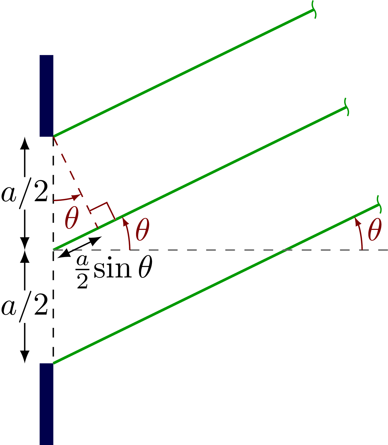
% DIFFRACTION - ONE SLIT - PATH DIFFERENCE close-up
\begin{tikzpicture}
\message{Diffraction, path difference (close-up)^^J}
\def\L{6.15} % distance between walls
\def\l{4.0} % path length
\def\H{4.3} % total wall height
\def\f{0.9} % fractional height of projection point
\def\t{0.15} % wall thickness
\def\a{2.5} % slit distance
\def\ang{26} % angle
\coordinate (T) at (0,\a/2);
\coordinate (B) at (0,-\a/2);
\coordinate (L) at (0,0);
\coordinate (R) at (\L,0);
\coordinate (I) at ({\a/2/tan(\ang)},0);
% LINES
\draw[mygreen,thick] (T) --++ (\ang:.8*\l) coordinate (PT); %node[midway,below=1,above left=-2] {$r_1$};
\draw[mygreen,thick] (B) --++ (\ang:\l) coordinate (PB); %node[midway,left=2,below right=-1] {$r_2$};
\draw[mygreen,thick] (L) --++ (\ang:.9*\l) coordinate (PR);
\draw[dashed] (T) -- (B);
\draw[mydarkred,dashed] (T) -- ($(L)!(T)!(PR)$) coordinate (M);
%\draw[black!60,dashed] (T) --++ (.20*\L,0) coordinate (TR);
\draw[black!60,dashed] (L) --++ (.6*\L,0) coordinate (LR);
%\draw[black!60,dashed] (B) --++ (.20*\L,0) coordinate (BR);
% LINE END
\lineend{PT}{\ang+70}
\lineend{PR}{\ang+70}
\lineend{PB}{\ang+70}
% ANGLES
\draw pic[mysmallarr,"$\theta$",mydarkred,draw=mydarkred,angle radius=20,angle eccentricity=1.3]
{angle = B--T--M}; %\contour{white}{}
\draw pic[mysmallarr,"$\theta$",mydarkred,draw=mydarkred,angle radius=24,angle eccentricity=1.2]
{angle = LR--L--PR};
\draw pic[mysmallarr,"$\theta$",mydarkred,draw=mydarkred,angle radius=24,angle eccentricity=1.2]
{angle = LR--I--PB};
\rightAngle{T}{M}{PR}{0.3}
% MEASURES
\draw[<->,black] (-2.1*\t,0) --++ (0,\a/2) node[midway,fill=white,inner sep=0.1] {$a/2$};
\draw[<->,black] (-2.1*\t,0) --++ (0,-\a/2) node[midway,fill=white,inner sep=0.1] {$a/2$};
\draw[<->,black] ([shift={({\ang-90}:0.1)}]L) -- ([shift={({\ang-90}:0.1)}]M)
node[midway,left=5,below right=-1]{$\frac{a}{2}\!\sin\theta$};
% WALL
\fill[wall]
(0,\a/2) rectangle (-\t,\H/2)
(0,-\a/2) rectangle (-\t,-\H/2);
\end{tikzpicture}
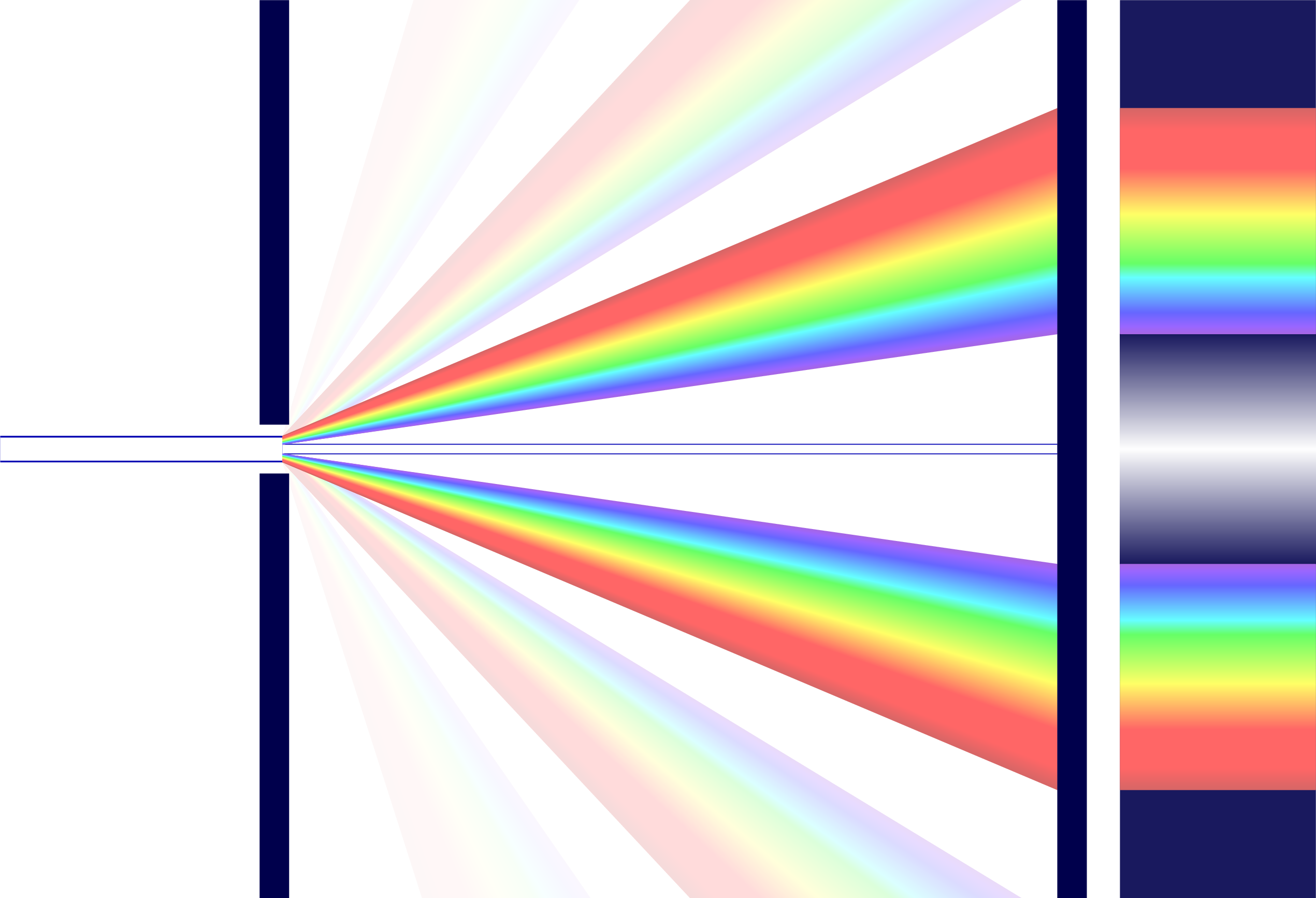
% DIFFRACTION - dispersion
\begin{tikzpicture}
\message{Diffraction, dispersion^^J}
\def\L{4.8} % distance between walls
\def\H{5.5} % total wall height
\def\l{5.5} % second/third order ray length
\def\t{0.18} % wall thickness
\def\a{0.3} % slit distance
\def\N{200} % number of rays in rainbow
\def\A{1.2} % band height
\def\ym{0.128*\H} % minimum y coordinate of 2nd order (violet)
\def\xb{1.08*\L} % band x position
% SHADE
\fill[myshadow]
(\xb,-\H/2) rectangle++ (\A,\H);
\fill[left color=myshadow,right color=myshadow,middle color=white,shading angle=0]
(\xb,-\ym) rectangle++ (\A,2*\ym);
% RAYS, THIRD & FOURTH ORDER
\message{ Third \& fourth order^^J}
\begin{scope}
\clip (0,-\H/2) rectangle++ (\L,\H);
\foreach \i [evaluate={\f=\i/\N;\lamb=410.+\f*320.;\dy=0.051*\f;\ang=31+\f*16;}] in {0,...,\N}{
\definecolor{tmpcol}{wave}{\lamb}
\colorlet{mycol}[rgb]{tmpcol}
\fill[mycol!3,line width=0.3] % third order
(0.05, 0.028+\dy) -- ( 25+\ang:\l) -- ( 25+\ang+1:\l) -- (0.05, 0.030+\dy)
(0.05,-0.028-\dy) -- (-25-\ang:\l) -- (-25-\ang+1:\l) -- (0.05,-0.030-\dy);
\fill[mycol!14,line width=0.3]% second order
(0.10, 0.028+\dy) -- ( \ang:\l) -- ( \ang+0.1:\l) -- (0.05, 0.030+\dy)
(0.10,-0.028-\dy) -- (-\ang:\l) -- (-\ang-0.1:\l) -- (0.05,-0.030-\dy);
}
\end{scope}
% RAYS, FIRST ORDER
\message{ First order^^J}
\draw[myblue,line width=4.6] (-0.35*\L,0) -- (0.05,0); % incoming white light
\draw[white, line width=4.0] (-0.35*\L,0) -- (0.05,0); % incoming white light
\draw[myblue,line width=1.8] (0.05,0) -- (\L,0);
\draw[white, line width=1.5] (0.05,0) -- (\L,0);
% RAYS, SECOND ORDER
\message{ Second order^^J}
\foreach \i [evaluate={\f=\i/\N;\lamb=410.+\f*320.;\dy=0.051*\f;
\y=\ym+\f*0.25*\H;}]in {0,...,\N}{
\definecolor{tmpcol}{wave}{\lamb}
\colorlet{mycol}[rgb]{tmpcol}
\fill[mycol!60,line width=0.3] % instead of smooth gradient, use many thin polygons
(0.05, 0.028+\dy) -- (\L, \y) -- (\L, \y+0.01) -- (0.05, 0.030+\dy)
(0.05,-0.028-\dy) -- (\L,-\y) -- (\L,-\y-0.01) -- (0.05,-0.030-\dy)
(\xb, \y) rectangle++ (\A, 0.01)
(\xb,-\y) rectangle++ (\A,-0.01);
}
% WALL
\fill[wall]
(\t/2,\a/2) rectangle (-\t/2,\H/2)
(\t/2,-\a/2) rectangle (-\t/2,-\H/2)
(\L,-\H/2) rectangle (\L+\t,\H/2);
\end{tikzpicture}
\end{document}
Click to download: optics_diffraction.tex • optics_diffraction.pdf
Open in Overleaf: optics_diffraction.tex