")


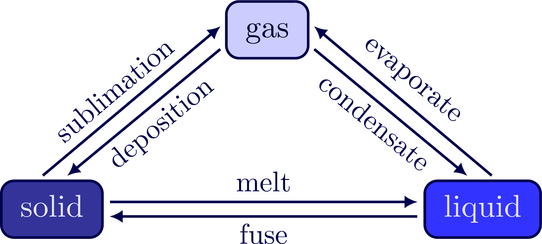
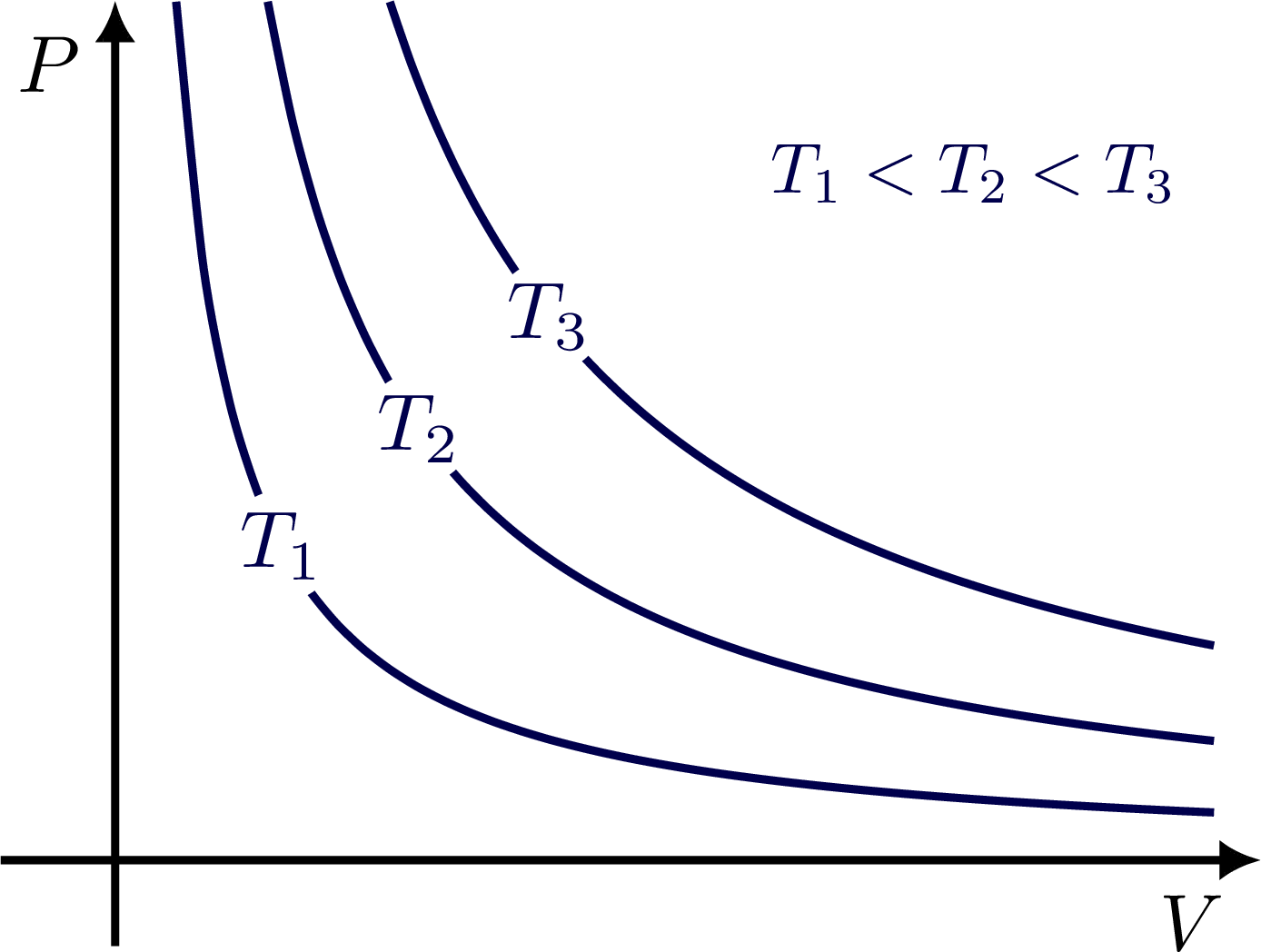
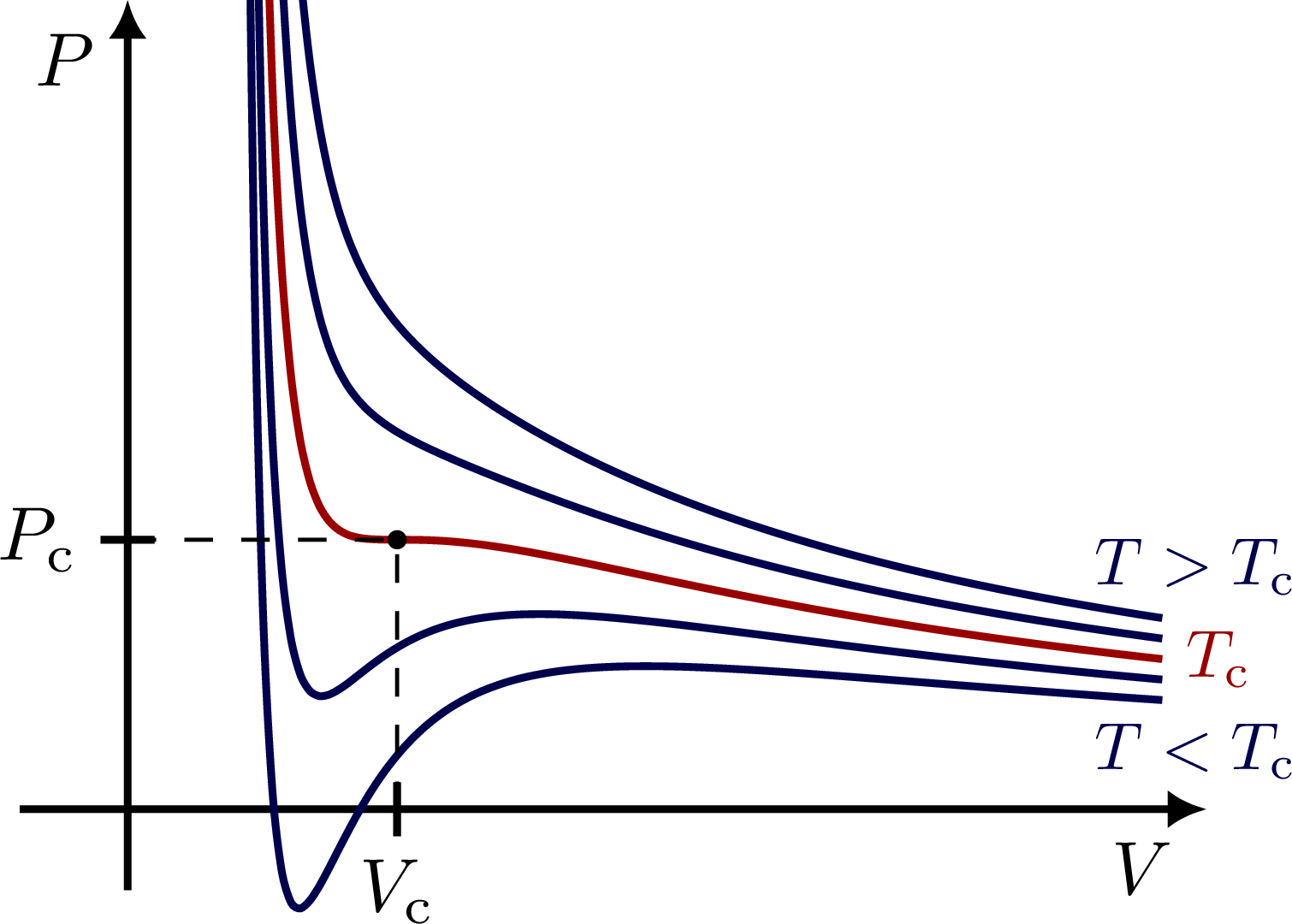
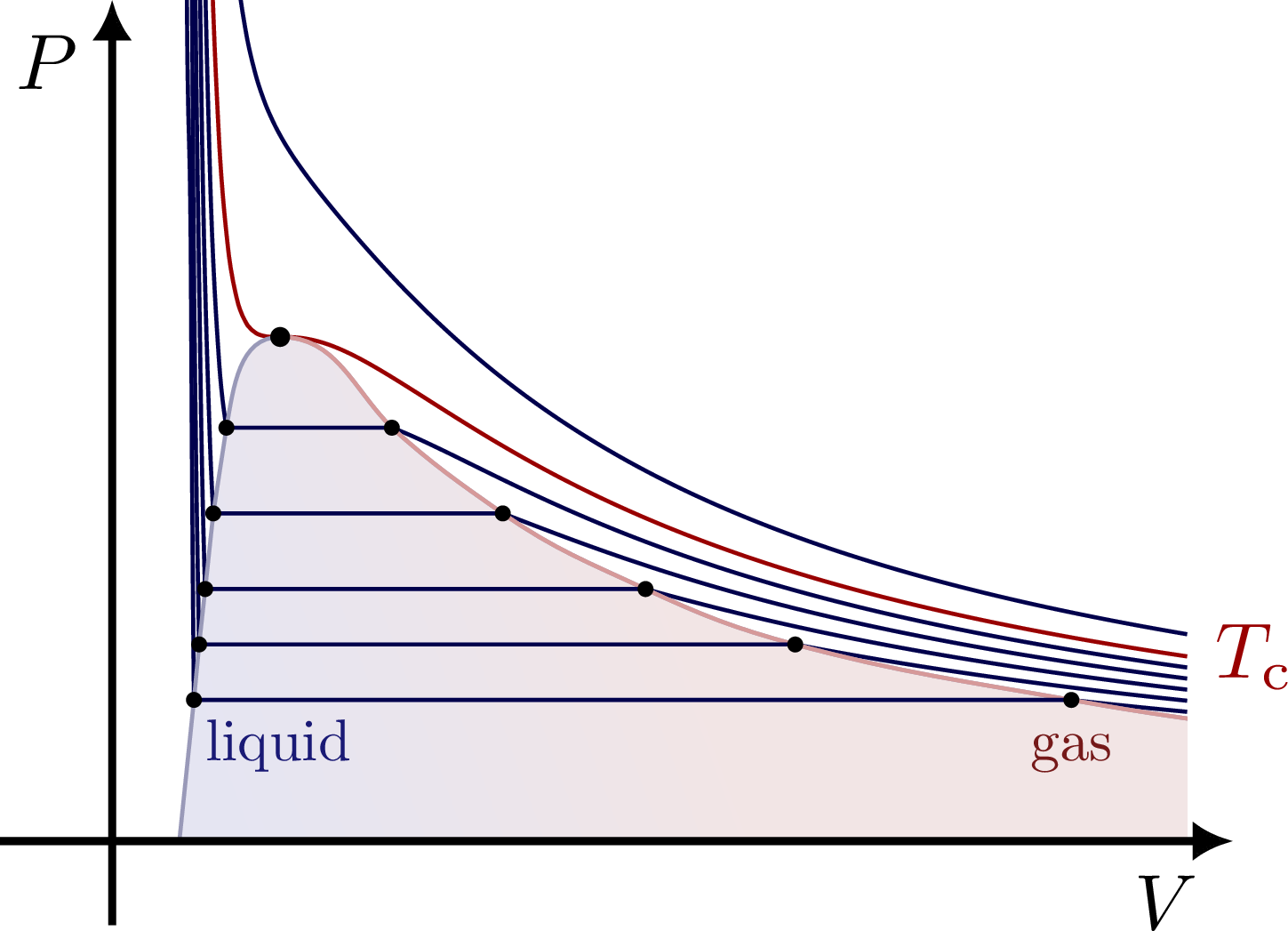
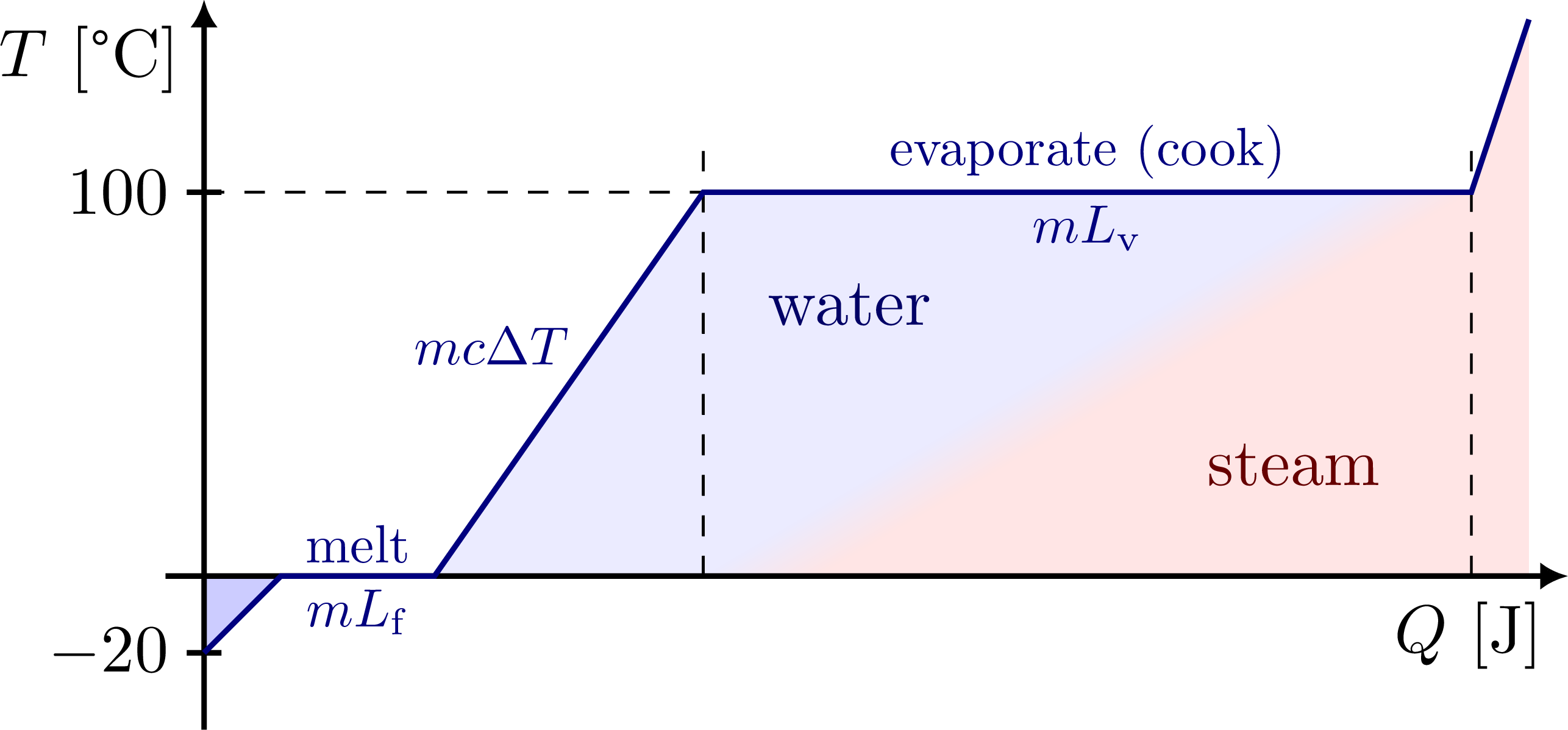
Phase transitions: phases of matter, PV diagrams, isotherms (ideal gas law & van der Waals), critical temperature, Maxwell’s construction, latent heat (converting ice into steam).
For more related figures, please see the Thermodynamics category.
Edit and compile if you like:
% Author: Izaak Neutelings (June, 2018)
\documentclass[border=3pt,tikz]{standalone}
\usepackage{ifthen}
\usepackage{siunitx}
\usepackage{tikz}
\usetikzlibrary{hobby} % for ..
\usetikzlibrary{arrows.meta} % to control arrow size
\tikzset{>={Latex[length=4,width=4]}} % for LaTeX arrow head
\usetikzlibrary{calc,intersections,decorations.markings}
\usepackage{siunitx}
\usepackage{xcolor} % for colored text
\colorlet{mylightblue}{blue!20}
\colorlet{myblue}{blue!50!black}
\colorlet{mydarkblue}{blue!30!black}
\colorlet{mylightred}{red!10}
\colorlet{myred}{red!50!black}
\colorlet{mydarkred}{red!60!black}
\colorlet{mydarkgreen}{green!30!black}
%\tikzstyle{midarr}=[decoration={markings,mark=at position 0.5 with {\arrow{stealth}}},postaction={decorate}]
\tikzset{
midarr/.style={decoration={markings,mark=at position #1 with {\arrow{stealth}}},postaction={decorate}},
midarr/.default=0.5
}
\def\tick#1#2{\draw[thick] (#1) ++ (#2:0.03*\ymax) --++ (#2-180:0.06*\ymax)}
\begin{document}
% PHASE TRANSITIONS
\begin{tikzpicture}[arrow/.style={->,thick,mydarkblue,shorten <=2,shorten >=2},
box/.style={thick,rounded corners=4,inner xsep=6,inner ysep=3}]
\message{Phase transitions^^J}
\node[blue!10!white,draw=mydarkblue,fill=blue!50!gray!80!black,box] (S) at (-2.4,0) {\strut solid};
\node[blue!10!white,draw=mydarkblue,fill=blue!80!white,box] (L) at (2.4,0) {\strut liquid};
\node[blue!20!black,draw=mydarkblue,fill=blue!20!white,box] (G) at (0,2) {\strut gas};
\draw[arrow,->] (S.8) -- (L.173) node[above,midway,scale=0.9] {melt};
\draw[arrow,->] (L.-173) -- (S.-8) node[below=-1pt,midway,scale=0.9] {fuse};
\draw[arrow,->] (S.115) -- (G.-190) node[left=2pt,above,midway,sloped,scale=0.9] {sublimation};
\draw[arrow,->] (G.-160) -- (S.70) node[left=-2pt,below=-1pt,midway,sloped,scale=0.9] {deposition};
\draw[arrow,->] (L.65) -- (G.10) node[left=2pt,above,midway,sloped,scale=0.9] {evaporate};
\draw[arrow,->] (G.-20) -- (L.110) node[left=2pt,below=-1pt,midway,sloped,scale=0.9] {condensate};
\end{tikzpicture}
% PHASE DIAGRAM
\begin{tikzpicture}[scale=0.4]
\message{Phase diagrams^^J}
\def\xtick#1#2{\draw[thick] (#1)++(0,.2) --++ (0,-.4) node[below=-.5pt,scale=0.7] {#2};}
\def\ytick#1#2{\draw[thick] (#1)++(.2,0) --++ (-.4,0) node[left=-.5pt,scale=0.7] {#2};}
% COORDINATES
\coordinate (O) at (0,0);
\coordinate (N1) at (2,10);
\coordinate (N2) at (11,10);
\coordinate (NE) at (12,10);
\coordinate (NW) at (0,10);
\coordinate (SE) at (12,0);
\coordinate (W) at (0,5);
\coordinate (S) at (6,0);
\coordinate (C) at (10.2,7.8); % critical
\coordinate (T) at (4,3); % triple
% PATHS
\def\SL{(T) -- (N1)}
\def\SG{(O) to[out=20,in=-120] (T)}
\def\LG{(T) to[out=20,in=-120] (C)}
\def\atm{(0,5.5) -- (12,5.5)}
\path[name path=SL] \SL;
\path[name path=LG] \LG;
\path[name path=atm] \atm;
% REGIONS
\fill[mylightblue] \SG -- (N1) -- (NW) -- cycle;
\fill[blue!5] \LG -- (N2) -- (N1) -- cycle;
\fill[mylightred] \LG -- (N2) -- (NE) -- (SE) -- \SG -- cycle;
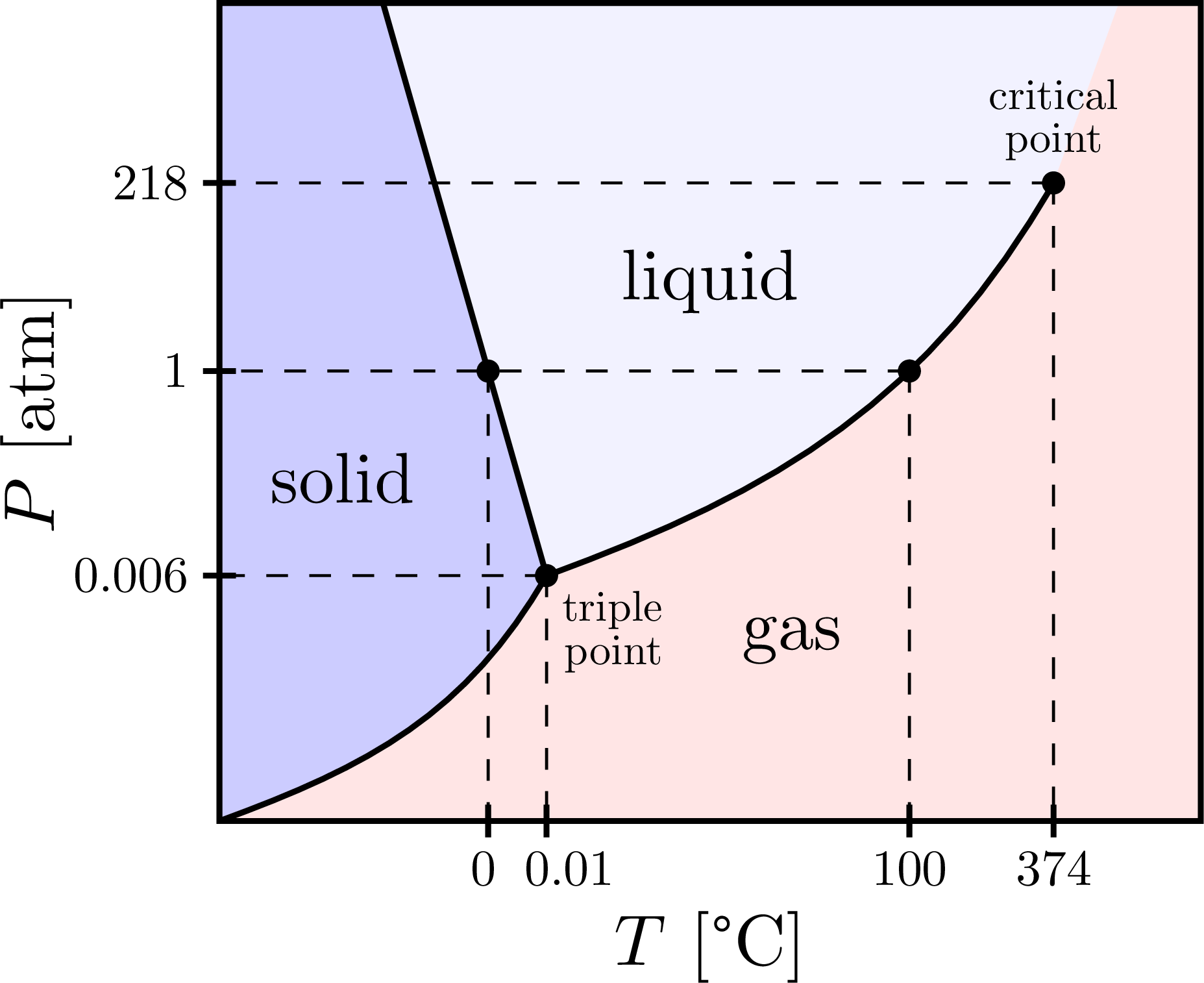
\node at (1.5,4.2) {solid};
\node at (7,2.2) {gas};
\node at (6,6.6) {liquid};
%% MIXED
%\shade[top color=mylightblue,bottom color=mylightred,shading angle=70]
% (10.4,7.7) -- (11.2,10) -- (10.8,10) -- (10.0,7.7) -- cycle;
% POINTS
\fill[black,name intersections={of=SL and atm,by=M}] (M) circle (4pt);
\fill[black,name intersections={of=LG and atm,by=B}] (B) circle (4pt);
\fill (T) circle (4pt) node[below right,scale=0.6,align=right] {triple\\[-2pt]point};
\fill (C) circle (4pt) node[above=1pt,scale=0.6,align=center] {critical\\[-2pt]point};
% LINES
\draw[thick] \SG;
\draw[thick] \LG;
\draw[thick] \SL;
\draw[dashed] (M) -- ($(M |- 0,0)$) coordinate (Mx);
\draw[dashed] (T) -- ($(T |- 0,0)$) coordinate (Tx);
\draw[dashed] (T) -- ($(T -| 0,0)$) coordinate (Ty);
\draw[dashed] (B) -- ($(B |- 0,0)$) coordinate (Bx);
\draw[dashed] (B) -- ($(B -| 0,0)$) coordinate (By);
\draw[dashed] (C) -- ($(C |- 0,0)$) coordinate (Cx);
\draw[dashed] (C) -- ($(C -| 0,0)$) coordinate (Cy);
% AXES
\draw[thick] (O) rectangle (NE);
\node[left=17pt,above,rotate=90] at (W) {$P$ [atm]};
\node[below=9pt] at (S) {$T$ [\si{\degree C}]};
\xtick{Mx}{\hspace{-2pt}0}
\xtick{Tx}{\hspace{9pt}0.01}
\ytick{Ty}{0.006}
\xtick{Bx}{100}
\ytick{By}{1}
\xtick{Cx}{374}
\ytick{Cy}{218}
\end{tikzpicture}
% PHASE DIAGRAM
\begin{tikzpicture}[scale=0.4]
\message{Phase diagrams 2^^J}
\def\xtick#1#2{\draw[thick] (#1)++(0,.2) --++ (0,-.4) node[below=-.5pt,scale=0.7] {#2};}
\def\ytick#1#2{\draw[thick] (#1)++(.2,0) --++ (-.4,0) node[left=-.5pt,scale=0.7] {#2};}
% COORDINATES
\coordinate (O) at (0,0);
\coordinate (N1) at (2,10);
\coordinate (N2) at (11,10);
\coordinate (NE) at (12,10);
\coordinate (NW) at (0,10);
\coordinate (SE) at (12,0);
\coordinate (W) at (0,5);
\coordinate (S) at (6,0);
\coordinate (C) at (10.2,7.8); % critical
\coordinate (T) at (4,3); % triple
% PATHS
\def\SL{(T) -- (N1)}
\def\SG{(O) to[out=20,in=-120] (T)}
\def\LG{(T) to[out=20,in=-120] (C)}
\def\atm{(0,5.5) -- (12,5.5)}
\path[name path=SL] \SL;
\path[name path=LG] \LG;
\path[name path=atm] \atm;
% REGIONS
\fill[mylightblue] \SG -- (N1) -- (NW) -- cycle;
\fill[blue!5] \LG -- (N2) -- (N1) -- cycle;
\fill[mylightred] \LG -- (N2) -- (NE) -- (SE) -- \SG -- cycle;
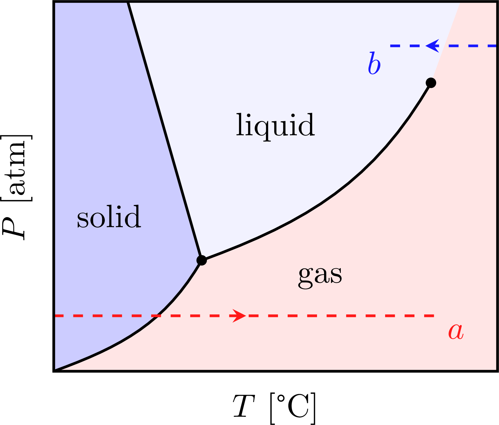
\node at (1.5,4.2) {solid};
\node at (7.2,2.5) {gas};
\node at (6,6.6) {liquid};
% POINTS
\fill (T) circle (4pt);
\fill (C) circle (4pt);
% LINES
\draw[thick] \SG;
\draw[thick] \LG;
\draw[thick] \SL;
\draw[dashed,red!90,thick,midarr]
(0,1.5) --++ (10.4,0) node[below right=-1] {$a$};
\draw[dashed,blue!90,thick,midarr=0.65]
(12,8.8) --++ (-3,0) node[below left=-2] {$b$};
% AXES
\draw[thick] (O) rectangle (NE);
\node[left=3pt,above,rotate=90] at (W) {$P$ [atm]};
\node[below=3pt] at (S) {$T$ [\si{\degree C}]};
\end{tikzpicture}
% PV diagram - isotherms
\begin{tikzpicture}
\message{PV diagram - isotherms^^J}
\def\tick{0.05*\xmax}
\def\xmax{4}
\def\ymax{3}
\def\N{40}
\def\isotherm#1#2{{ 1.6*#2/#1 }}
% AXIS
\draw[->,thick] (0,-0.1*\ymax) -- (0,\ymax)
node[anchor=north east,inner sep=4,scale=0.8] {$P$};
\draw[->,thick] (-0.1*\xmax,0) -- (\xmax,0)
node[anchor=north east,inner sep=4,scale=0.8] {$V$};
% ISOTHERMS
\path[name path=line] (0,.2*\ymax) -- (.7*\xmax,\ymax);
\foreach \i/\T in {1/0.4,2/1,3/1.8}{
\draw[mydarkblue,thick,name path=isotherm\i,
variable=\x,domain={\isotherm{\ymax}{\T}}:{.96*\xmax},samples=\N,smooth]
plot (\x,\isotherm{\x}{\T});
\node[mydarkblue,fill=white,circle,inner sep=0.2,scale=0.8,
name intersections={of=line and isotherm\i,by=T\i}]
at (T\i) {$T_\i$};
}
% LABELS
\node[mydarkblue,scale=0.7] at (.75*\xmax,.8*\ymax) {$T_1<T_2<T_3$};
\end{tikzpicture}
% PV diagram - van der Waals isotherms
\begin{tikzpicture}
\message{PV diagram - van der Waals isotherms^^J}
\def\tick{0.05*\xmax}
\def\xmax{4}
\def\ymax{3}
\def\N{100}
\def\s{1}
\def\R{4}
\def\isotherm#1#2{{ (8*#2)/(3*#1-1) - 3/(#1*#1) }} % reduced equation of state
\coordinate (C) at (\s,1);
% AXIS
\draw[->,thick] (0,-0.1*\ymax) -- (0,\ymax)
node[anchor=north east,inner sep=4,scale=0.8] {$P$};
\draw[->,thick] (-0.1*\xmax,0) -- (\xmax,0)
node[anchor=north east,inner sep=4,scale=0.8] {$V$};
% ISOTHERMS
\begin{scope}
\clip (-0.2*\xmax,-0.2*\ymax) rectangle (1.11*\xmax,\ymax);
\foreach \i/\T in {1/0.8,2/0.9,3/1.0,4/1.1,5/1.2}{
\ifthenelse{\lengthtest{\T pt = 1.0 pt}}{
\draw[mydarkred,thick,variable=\x,domain=0.36:{.96*\xmax/\s},range=0:1,samples=\N,smooth]
plot (\s*\x,\isotherm{\x}{\T}) coordinate (EC);
}{
\draw[mydarkblue,thick,variable=\x,domain=0.36:{.96*\xmax/\s},range=0:1,samples=\N,smooth]
plot (\s*\x,\isotherm{\x}{\T}) coordinate (E\i);
}
}
\end{scope}
% LABELS
\node[mydarkblue,scale=0.7,right=5,below] at (E1) {$T<T_\text{c}$};
\node[mydarkred,right,scale=0.7] at (EC) {$T_\text{c}$};
\node[mydarkblue,scale=0.7,right=5,above] at (E5) {$T>T_\text{c}$};
% CRITICAL POINT
\fill[black] (C) circle (1pt);
\draw[dashed] (0,1) -- (C) -- (\s,0);
\draw[thick] (\s,\tick/2) --++ (0,-\tick) node[below=-.5pt,scale=0.8] {$V_\text{c}$};
\draw[thick] (\tick/2,1) --++ (-\tick,0) node[left=-.5pt,scale=0.8] {$P_\text{c}$};
\end{tikzpicture}
% PV diagram - Maxwell construction
\begin{tikzpicture}
\message{PV diagram - Maxwell construction^^J}
\def\xmax{4}
\def\ymax{3}
\def\N{110}
\def\s{0.6}
\def\A{1.8}
\def\isotherm#1#2{{ \A*(8*#2)/(3*#1-1) - 3*\A/(#1*#1) }} % reduced equation of state
\coordinate (C) at (\s,\A);
% LINE
\foreach \i/\T/\pe in {0/.75/.28,1/.8/.39,2/.85/.5,3/.9/.65,4/.95/.82,5/1.0/1,6/1.1/1}{
\begin{scope}
\clip (-0.15*\xmax,0) rectangle (1.10*\xmax,\ymax);
\ifthenelse{\i = 5}{
\draw[mydarkred,variable=\x,domain=0.36:{.96*\xmax/\s},range=0:1,samples=\N,smooth,name path=isotherm]
plot (\s*\x,\isotherm{\x}{\T}) node[mydarkred,right,scale=0.8] {$T_\text{c}$};
}{
\draw[mydarkblue,variable=\x,domain=0.36:{.96*\xmax/\s},range=0:1,samples=\N,smooth,name path=isotherm]
plot (\s*\x,\isotherm{\x}{\T});
}
\ifthenelse{\i < 5}{ %\lengthtest{\pe pt < 1 pt}
\path[name path={pe}] (0,\A*\pe) --++ ({.96*\xmax/\s},0);
\path[name intersections={of=isotherm and pe,name=pe\i}];
}
\end{scope}
}
\begin{scope}
\clip (0,0) rectangle (.96*\xmax,.96*\ymax);
\fill[top color=myblue!10,bottom color=myred!10,middle color=myred!10,shading angle=110,
draw=mydarkblue!40,thin,use Hobby shortcut]
(.06*\xmax,0) -- (pe0-1) -- (pe1-1) -- (pe2-1) -- (pe3-1) --
(pe4-1) to[out=80,in=180]
(C) to[out=0,in=135]
(pe4-3) to[out=-42,in=145]
(pe3-3) to[out=-35,in=155]
(pe2-3) to[out=-25,in=165]
(pe1-3) to[out=-15,in=170]
(pe0-3) to[out=-10,in=172]
(.97*\xmax,.144*\ymax) |- (0,0);
\draw[mydarkred!40,thin,use Hobby shortcut]
(C) to[out=0,in=135]
(pe4-3) to[out=-42,in=145]
(pe3-3) to[out=-35,in=155]
(pe2-3) to[out=-25,in=165]
(pe1-3) to[out=-15,in=170]
(pe0-3) to[out=-10,in=172]
(.97*\xmax,.144*\ymax) |- (0,0);
\end{scope}
\node[blue!40!black!90,below right=-1,scale=0.6] at (pe0-1) {\strut liquid};
\node[red!40!black!90,below=-1,scale=0.6] at (pe0-3) {\strut gas};
% MAXWELL CONSTRUCTION
\fill (C) circle (1pt);
\foreach \i in {0,1,2,3,4}{
\draw[thin,mydarkblue] (pe\i-1) -- (pe\i-3);
\fill[black] (pe\i-3) circle (.8pt);
\fill[black] (pe\i-1) circle (.8pt);
}
% AXIS
\draw[->,thick] (0,-0.1*\ymax) -- (0,\ymax)
node[anchor=north east,inner sep=4,scale=0.8] {$P$};
\draw[->,thick] (-0.1*\xmax,0) -- (\xmax,0)
node[anchor=north east,inner sep=4,scale=0.8] {$V$};
\end{tikzpicture}
%%% PV diagram - van der Waals isotherms (PGF)
%%\begin{tikzpicture}
%% \def\N{40}
%% \def\xmax{4}
%% \def\ymax{3}
%% \begin{axis}[every axis plot post/.append style={
%% mark=none,domain=0.1:\xmax,samples=\N,smooth},
%% xmin=(-.05*\xmax), xmax=(1.05*\xmax),
%% ymin=(-.08*\ymax), ymax=(1.08*\ymax),
%% restrict y to domain=-\ymax:\ymax,
%% axis lines=middle,
%% axis line style=thick,
%% ticks=none,
%% xlabel={$V$},
%% ylabel={$P$},
%% xlabel style={at={(rel axis cs:0.5,0)},below=-2pt,font=\small},
%% ylabel style={at={(rel axis cs:-0.1,0.5)},rotate=90},
%% width=9cm, height=7cm,
%% %clip=false
%% ]
%% \addplot plot {8*1/(3*x-1) - 3/x^2};
%%
%% \addplot[domain=0:\ymax, samples=90] {max(0,8*2/(3*x-1) - 3/x^2)};
%%
%% \end{axis}
%%\end{tikzpicture}
% PHASE TRANSITIONS - ice -> water -> steam
\begin{tikzpicture}
\message{Phase transition of ice -> water -> steam^^J}
\def\ymin{-0.8}
\def\ymax{3}
\def\xmin{-0.2}
\def\xmax{7}
\def\t{0.3} % water/steam transition zone
\def\ang{30.4} % angle gradient
\coordinate (O) at (0,0);
\coordinate (I) at (0.0,-0.4); % ice
\coordinate (M) at (0.4,0.0); % melting
\coordinate (W) at (1.2,0.0); % water
\coordinate (E) at (2.6,2,0); % evaporate
\coordinate (S) at (6.6,2.0); % steam
\coordinate (F) at (6.9,2.9); % final
\coordinate (Ex) at ($(E|-O)$); % x evaporation
\coordinate (Ey) at ($(E-|O)$); % y evaporation
\coordinate (Sx) at ($(S|-O)$); % x steam
\coordinate (Fx) at ($(F|-O)$);
% AREA
\fill[mylightblue] (O) -- (I) -- (M) -- cycle;
\fill[blue!8] (W) -- (Ex) -- (S) -- (E) -- cycle;
\fill[mylightred] (Ex) -- (S) -- (F) -- (Fx) -- cycle;
\begin{scope} % fade/gradient border
\clip (Ex) -- (Sx) -- (S) -- (E) -- cycle; % clip gradient rectangle
\draw[draw=none,transform canvas={rotate=\ang},top color=blue!8,bottom color=mylightred,shading angle=0]
({2.6*cos(\ang)},{-2.6*sin(\ang)-\t}) rectangle++(0.65*\xmax,\t); % diagonal border
\end{scope}
\node[blue!40!black,left=4,below right=10] at (E) {water};
\node[red!40!black,above left=10] at (Sx) {steam};
% AXES
\draw[->,thick] (0,\ymin) -- (0,\ymax) node[below left=0] {$T$ [\si{\degree C}]};
\draw[->,thick] (\xmin,0) -- (\xmax+0.1,0) node[below left=0] {$Q$ [J]}; %[\si{J}]
\draw[dashed] (Ex) -- (E) --++ (0,0.1*\ymax);
\draw[dashed] (Ey) -- (E);
\draw[dashed] (Sx) -- (S) --++ (0,0.1*\ymax);
\tick{I}{0} node[left=-1] {$-20$};
\tick{Ey}{0} node[left=-1] {$100$};
\draw[dashed] (E) -- (Ex);
\draw[myblue,thick]
(I) -- (M) -- (W)
node[midway,above=-1,scale=0.8] {melt}
node[midway,below=-1,scale=0.8] {$mL_\mathrm{f}$} --
(E)
node[pos=0.6,left=1,scale=0.8] {$mc\Delta T$} --
(S)
node[midway,above=-1,scale=0.8] {evaporate (cook)}
node[midway,below=-1,scale=0.8] {$mL_\mathrm{v}$} --
(F);
\end{tikzpicture}
\end{document}
Click to download: phase_transitions.tex • phase_transitions.pdfOpen in Overleaf: phase_transitions.tex


I think there is an error in compiling due to graph 3.
Hey Jet, thank you for the heads up! HTML does not like ‘<', but it should be fixed now. Cheers, Izaak
Hello,
in the heating curve plot, I saw the following:
\coordinate (Ex) at ($(EI-O)$); % x evaporation
\coordinate (Ey) at ($(E-IO)$); % y evaporation
I couldn’t find in the documentation what the EI-O and the E-IO do to the coordinates. Would you be able to explain briefly? I studied the output, but could not make sense of what the question is doing.
Thank you,
J.
Hi,
It is explained in Section 13.3 in the manual, have a look here:
https://tikz.dev/tikz-coordinates#tikz-lib-calc
Maybe it’s more clear from this simple example:
\documentclass[border=3pt,tikz]{standalone}
\tikzset{>=latex} % for LaTeX arrow head
\usepackage{xcolor}
\colorlet{mygreen}{green!80!black}
\begin{document}

% PROJECT COORDINATES
\begin{tikzpicture}[scale=0.8]
   \draw[black!40,step=0.5] (0,0) grid (4,3);
   \draw[->,thick] (0,0) -- (4.5,0); % x axis
   \draw[->,thick] (0,0) -- (0,3.5); % y axis
   \fill[black] (0,0) coordinate(O) circle(2pt) node[below left] {$O$};
   \fill[mygreen] (3,2) coordinate(R) circle(2pt) node[above right] {$R$};
   \fill[blue] (R|-O) coordinate(X) circle(2pt) node[below] {$X$}; % project on horizontal line through O
   \fill[red] (R-|O) coordinate(Y) circle(2pt) node[left] {$Y$}; % project on vertical line through O
   \draw[->,thick,mygreen] (R) -- (X);
   \draw[->,thick,red] (R) -- (Y);
\end{tikzpicture}

% PROJECT LINES
\begin{tikzpicture}[scale=0.8]
  \draw[black!40,step=0.5] (0,0) grid (4,3);
  \draw[->,thick] (0,0) -- (4.5,0); % x axis
  \draw[->,thick] (0,0) -- (0,3.5); % y axis
  \fill[black] (0,0) coordinate(O) circle(2pt) node[below left] {$O$};
  \fill[mygreen] (3,2) coordinate(A) circle(2pt) node[above right] {$A$};
  \fill[blue] (1,1) coordinate(B) circle(2pt) node[above right] {$B$};
   \draw[->,thick,mygreen] (A) -| (B); % horizontal, then vertical
   \draw[->,thick,blue] (A) |- (B); % vertical, then horizontal
\end{tikzpicture}

\end{document}
Basically
(R|-O)projects the(R)coordinate onto a horizontal line line through(O), while(R|-O)projects(R)onto a vertical line line through(O). I do not think the dollar signs are actually needed in this case (they are syntax for thecalclibrary to operate on coordinates, like subtraction, addition, scaling, interpolation, etc.).In the second example, you see that you can also use
|-and-|to draw a line with a 90° angle between two coordinates:-|is “horizontal, then vertical”,|-is “vertical, then horizontal”.Cheers,
Izaak
Hi everyone,
Could someone assist me with creating a T-V thermodynamic diagram using TikZ? I would like the diagram to include the following elements:
Isocoric Lines (constant volume lines)
Isobaric Lines (constant pressure lines)
Shaded regions to represent the liquid phase, saturated phase, and vapor phase.
I can provide a reference image for clarity if needed.
Thank you for your help!
Best regards,