Punctuated equilibrium

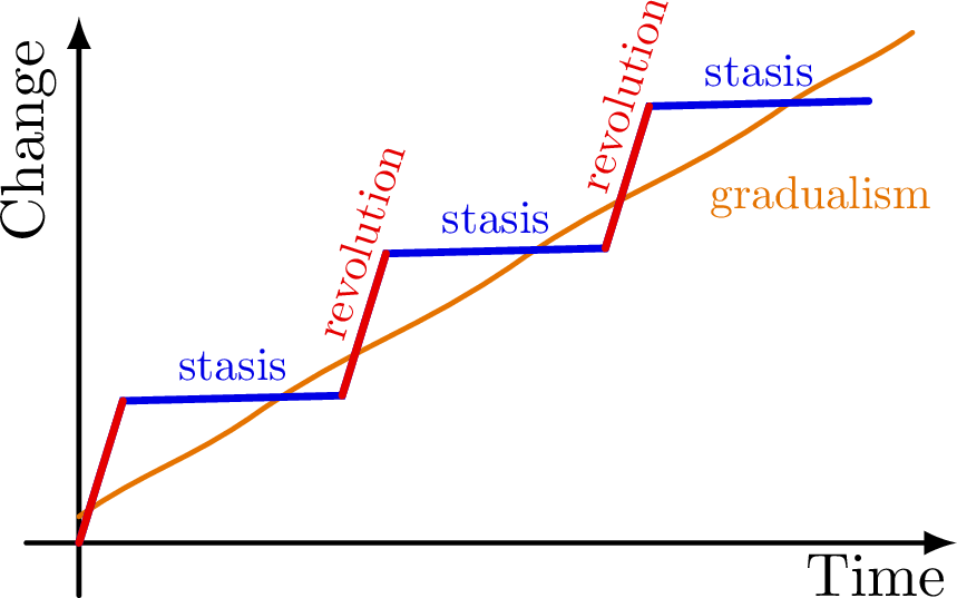
Intuitive graph of evolutionary changes over time, comparing gradualism (constant, small changes) versus punctuated equilibrium (long periods of stasis with occasional short periods of rapid change), sometimes summarized as “evolution versus revolution” or “creeps vs. jerks”. Inspired by Robert Sapolsky’s lecture on Human Behavioral Biology. Also see Sapolsky’s behavioral diagram.

The structure of punctuated equilibrium is similar to Thomas Kuhn’s idea of how science progresses with sudden paradigm shifts as opposed to slow, steady improvements of models (see the Stanford Encyclopedia of Philosophy).

Edit and compile if you like:

% Author: Izaak Neutelings (December 2020)
\documentclass[border=3pt,tikz]{standalone}
\usepackage{amsmath}
\usepackage{tikz}
\usepackage{physics}
\usetikzlibrary{calc}
\tikzset{>=latex} % for LaTeX arrow head
\usepackage{xcolor}
\colorlet{veccol}{green!45!black}
\colorlet{myred}{red!90!black}
\colorlet{myblue}{blue!90!black}
\colorlet{myorange}{orange!90!black}
\colorlet{mypurple}{blue!50!red!80!black!80}
\tikzstyle{vector}=[->,very thick,veccol]
\usetikzlibrary{arrows.meta}

\begin{document}


% TWO VECTORS SUM
\begin{tikzpicture}[line cap=round] %[xscale=4,yscale=2]
  \def\xmax{5}
  \def\ymax{3}
  \def\xb{0.95*\xmax}
  \def\ya{0.05*\ymax}
  \def\yb{0.97*\ymax}
  \def\y#1{{\ya+(\yb-\ya)/(\xb)*#1}}
  \draw[->,thick] (-0.1*\ymax,0) -- (\xmax,0) node[below left=-2] {Time};
  \draw[->,thick] (0,-0.1*\ymax) -- (0,\ymax) node[above left,rotate=90] {Change};
  \draw[thick,myorange]
    (0,\ya)
      to[out=35,in=-145] (0.2*\xmax,\y{0.2*\xmax})
      to[out=35,in=-145] (0.5*\xmax,\y{0.5*\xmax})
      to[out=35,in=-145] (0.8*\xmax,\y{0.8*\xmax}) %node[below right,scale=0.75,myorange] {gradualism};
      to[out=35,in=-145] (\xb,\yb);
  \node[below right,scale=0.75,myorange] at (0.7*\xmax,\y{0.7*\xmax}) {gradualism};
  \draw[very thick,myblue]
    (0,0) coordinate (O) --++
    (0.05*\xmax,0.27*\ymax) coordinate (A1) --++
    (0.25*\xmax,0.01*\ymax) coordinate (A2) node[midway,above,scale=0.75] {stasis} --++
    (0.05*\xmax,0.27*\ymax) coordinate (B1) --++ %node[above,scale=0.5,rotate=60] {revolution} --++
    (0.25*\xmax,0.01*\ymax) coordinate (B2) node[midway,above,scale=0.75] {stasis} --++
    (0.05*\xmax,0.27*\ymax) coordinate (C1) --++ % node[above,scale=0.5,rotate=60] {revolution}
    (0.25*\xmax,0.01*\ymax) coordinate (C2) node[midway,above,scale=0.75] {stasis};
  \draw[very thick,myred]
    (O) -- (A1)
    (A2) node[left=3,above right=5,scale=0.75,rotate=72] {revolution} -- (B1)
    (B2) node[left=3,above right=5,scale=0.75,rotate=72] {revolution} -- (C1);
  
\end{tikzpicture}


\end{document}