Pzeta definition

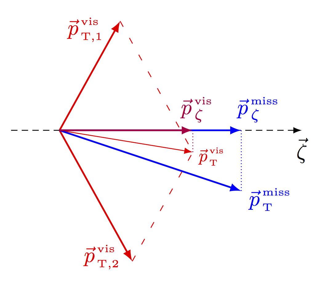
Construction of the P_ζ variable to help discriminate against backgrounds in H → 𝜏𝜏 analyses in proton-proton collision data at the CMS detector. Inspired by Jang Dongwook’s dissertation.

Edit and compile if you like:

% Basic drawings
% https://www.sharelatex.com/blog/2013/08/27/tikz-series-pt1.html
% https://www.tug.org/TUGboat/tb29-1/tb91walczak.pdf
\documentclass{article}
\usepackage{amsmath}
\usepackage{tikz}
\tikzset{>=latex} % for LaTeX arrow head
\usetikzlibrary{calc} % to add coordinates
\newcommand*{\vv}[1]{\vec{\mkern0mu#1}} % correct misalignment
%\newcommand{\sq}{\medmuskip=1mu \thinmuskip=1mu \thickmuskip=1mu} % squeeze

% split figures into pages
\usepackage[active,tightpage]{preview}
\PreviewEnvironment{tikzpicture}
\setlength\PreviewBorder{5pt}%

\begin{document}



% PZETA
\begin{tikzpicture}
  
  % vector labels
  \def\pTM{\vv{p}^\text{\tiny\,miss}_\text{\tiny\,T}}
  \def\pT{ \vv{p}^\text{\tiny\,vis}_\text{\tiny\,T}}
  \def\pTA{\vv{p}^\text{\tiny\,vis}_\text{\tiny\,T,1}} %$\ell$
  \def\pTB{\vv{p}^\text{\tiny\,vis}_\text{\tiny\,T,2}} %$\tau_\text{h}$
  
  % define point
  \coordinate (O)  at (0.0, 0.0);
  \coordinate (Z)  at (4.0, 0.0);
  \coordinate (A)  at (1.0, 1.8);
  \coordinate (B)  at (1.2,-2.16);
  \coordinate (M)  at (3.0,-1.0);
  \coordinate (AB) at ($(A)+(B)$);
  \path let \p{AB}=(AB) in coordinate (P) at (\x{AB},0); % projection
  \path let \p{M} =(M)  in coordinate (Q) at (\x{M},0); % projection
  
  % axis
  \draw[->,densely dashed]
    (-0.8,0) -- (Z)
    node[at end,below] {$\vv{\zeta}$};
    %node[at end,below,scale=0.7] {bisector $\vv{\zeta}$};
  
  % visible vectors
  \draw[->,thick,color=red]
    (O) -- (A)
    node[below=4pt,left=4pt,color=red] {$\pTA$};
  \draw[->,thick,color=red]
    (O) -- (B)
    node[above=2pt,left=2pt,color=red] {$\pTB$};
  \draw[->,color=red]
    (O) -- (AB)
    node[below=2pt,right,color=red,scale=0.8] {$\pT$};
  \draw[->,thick,color=blue]
    (O) -- (M)
    node[below=4pt,right,color=blue] {$\pTM$};
  
  % helplines
  \draw[loosely dashed,color=red]
    (A) -- (AB);
  \draw[loosely dashed,color=red]
    (B) -- (AB);
  \draw[densely dotted,color=purple]
    (AB) -- (P);
  \draw[densely dotted,color=blue]
    (M) -- (Q);
  
  % vector sum
  \draw[->,thick,color=blue]
    (O) -- (Q)
    node[right=8pt,above,color=blue] {$\vv{p}^\text{\tiny\,miss}_{\tiny\,\zeta}$};
  \draw[->,thick,color=purple]
    (O) -- (P)
    node[right=2pt,above,color=purple] {$\vv{p}^\text{\tiny\,vis}_{\tiny\,\zeta}$};
      
\end{tikzpicture}



%% PZETA VIS
%\begin{tikzpicture}
%  
%  % vector labels
%  \def\pT{ \vv{p}^\text{\tiny\,vis}_\text{\tiny\,T}}
%  \def\pTA{\vv{p}^\text{\tiny\,vis}_\text{\tiny\,T,1}}
%  \def\pTB{\vv{p}^\text{\tiny\,vis}_\text{\tiny\,T,2}}
%  
%  % define point
%  \coordinate (O)  at (0.0, 0.0);
%  \coordinate (Z)  at (3.5, 0.0);
%  \coordinate (A)  at (1.0, 1.8);
%  \coordinate (B)  at (1.2,-2.16);
%  \coordinate (AB) at ($(A)+(B)$);
%  \path let \p{AB}=(AB) in coordinate (P) at (\x{AB},0); % projection
%  
%  % axis
%  \draw[->,thick,dashed]
%    (-0.8,0) -- (Z)
%    node[at end,below] {$\vv{\zeta}$};
%  
%  % main vectors
%  \draw[->,thick,color=red]
%    (O) -- (A)
%    node[below=4pt,left=4pt,color=red] {$\pTA$};
%  \draw[->,thick,color=red]
%    (O) -- (B)
%    node[above=2pt,left=2pt,color=red] {$\pTB$};
%  \draw[->,color=red]
%    (O) -- (AB)
%    node[below=4pt,right,color=red,scale=1] {$\pT$}; %{$\sq\pTA+\,\pTB$};
%  
%  % helplines
%  \draw[dashed,color=red]
%    (A) -- (AB);
%  \draw[dashed,color=red]
%    (B) -- (AB);
%  \draw[dashed,color=purple]
%    (AB) -- (P);
%
%  % vector sum
%  \draw[->,thick,color=purple]
%    (O) -- (P)
%    node[right=4pt,above,color=purple] {$\vv{p}^\text{\tiny\,vis}_{\tiny\,\zeta}$};
%      
%\end{tikzpicture}



\end{document}