")


Standing waves in a open and half-closed pipes. Also see standing waves in a flute, traveling waves in air, and more related figures in the Music category.
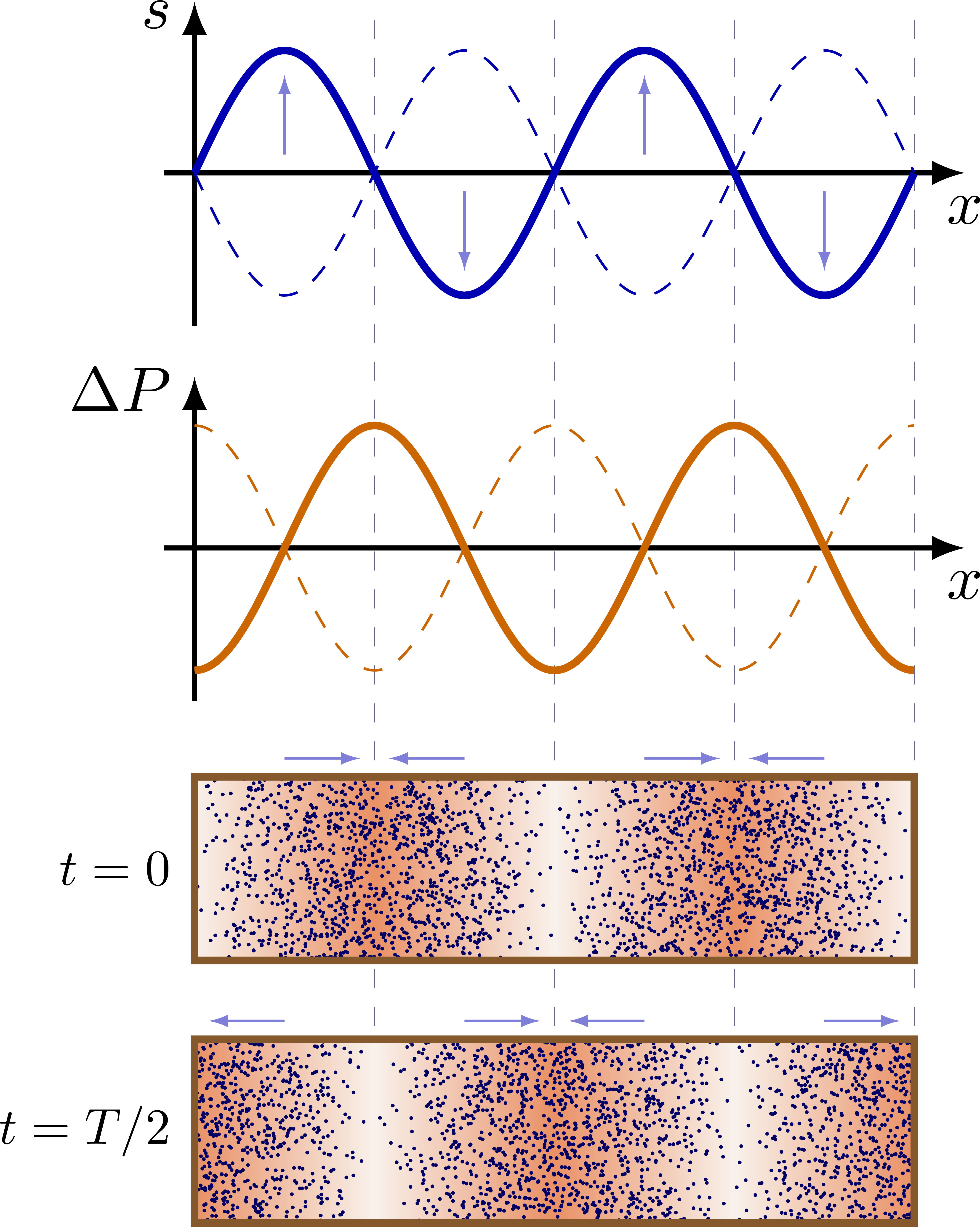
Pressure and displacement
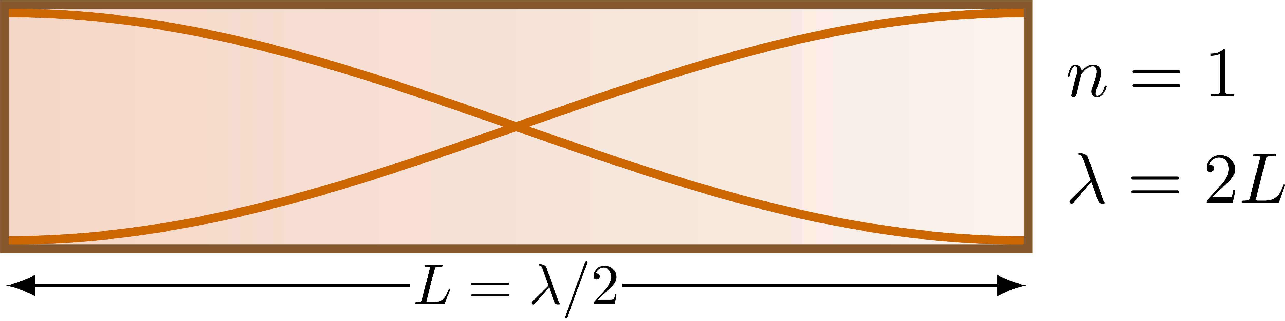
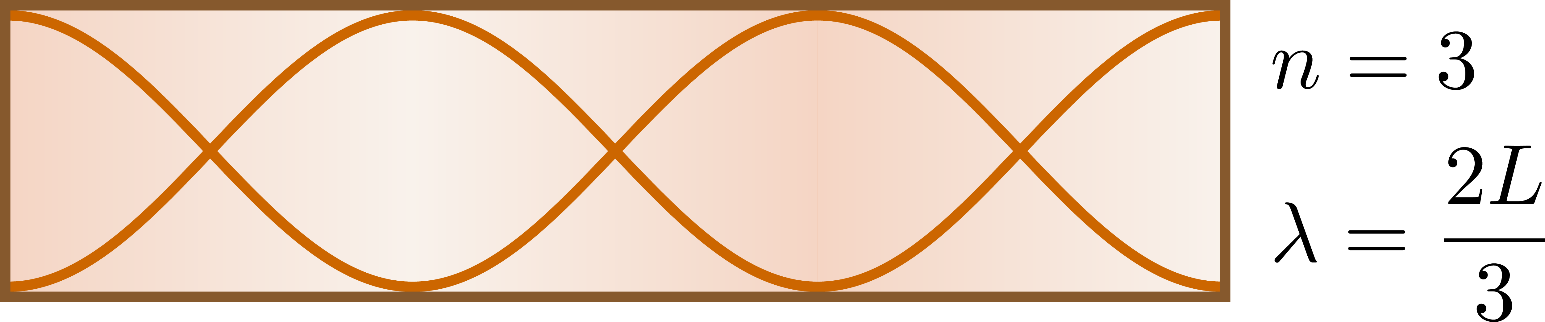
Closed pipe


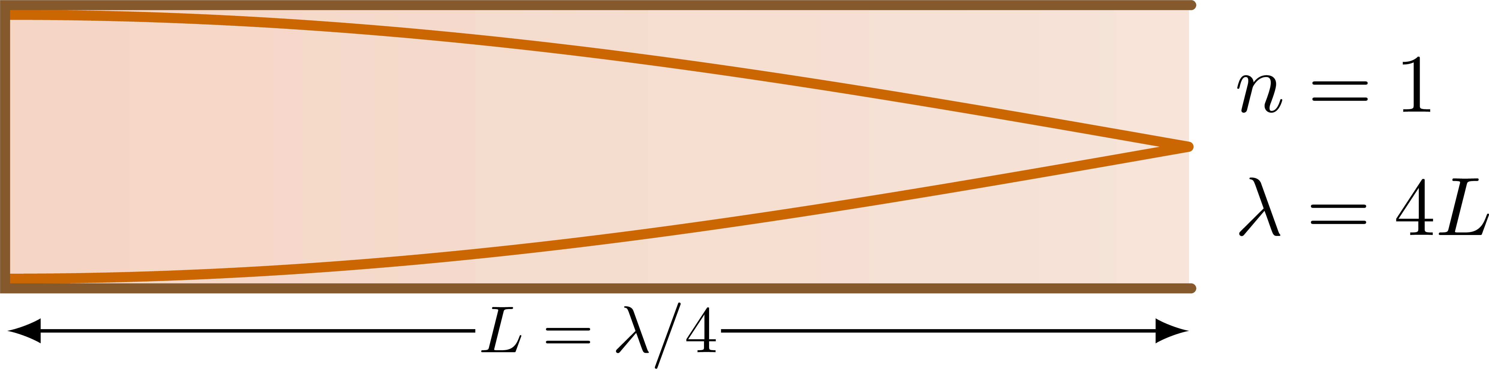
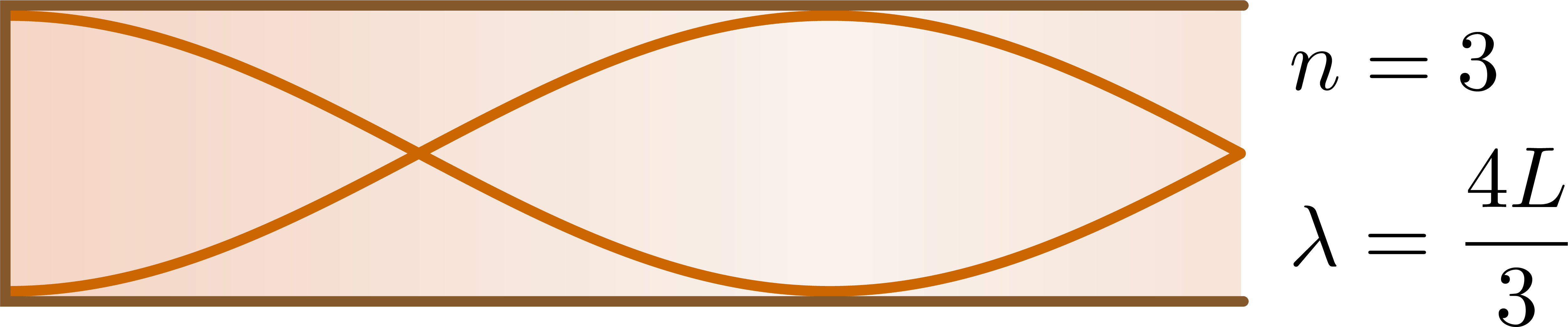
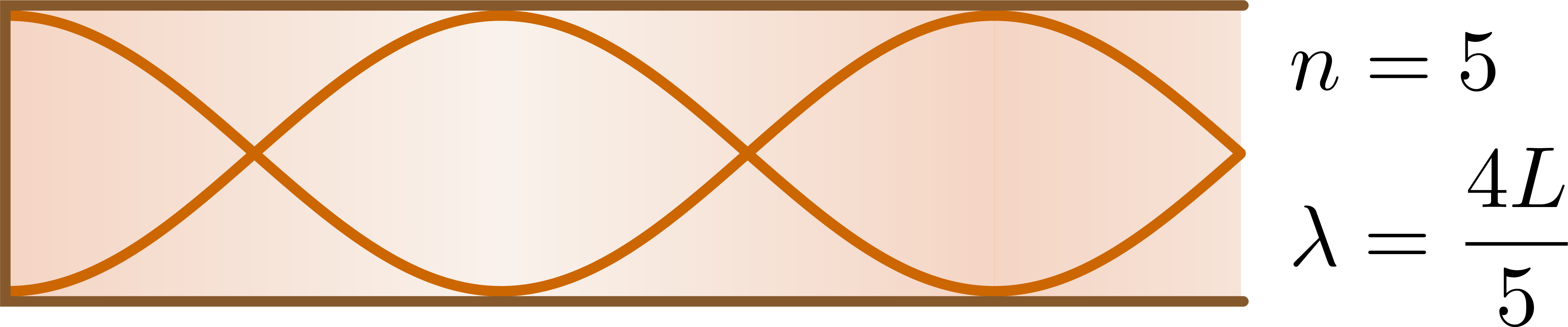
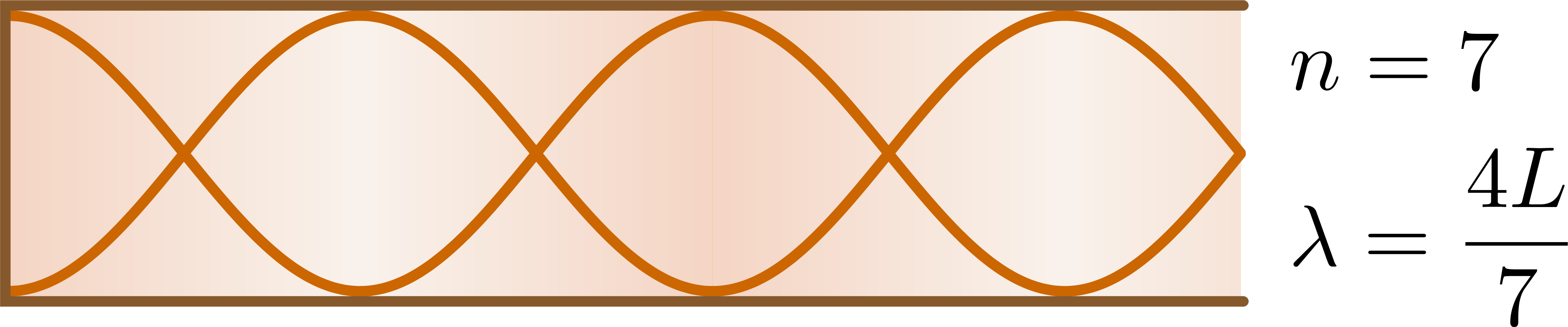
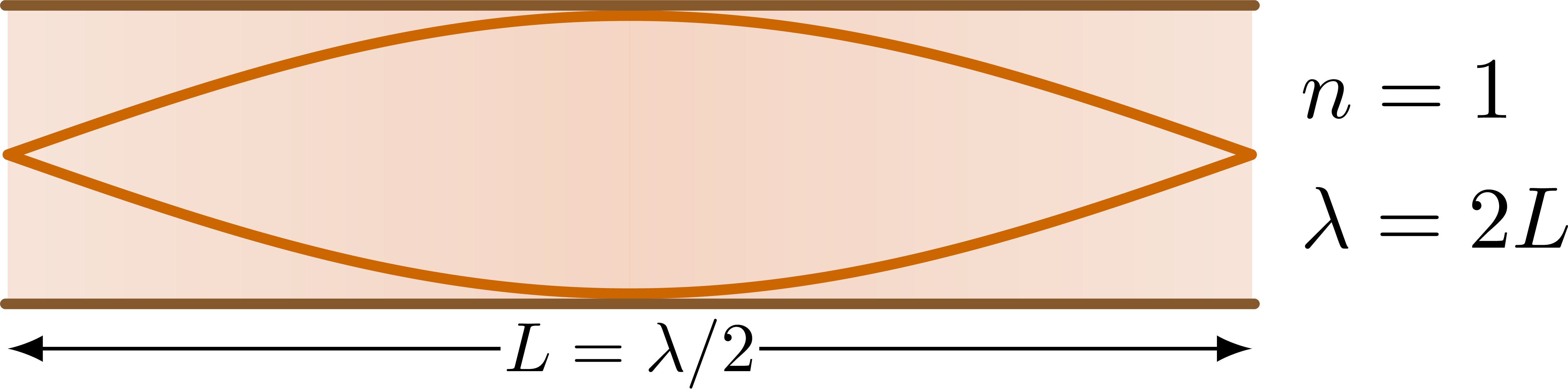
Half-open pipe
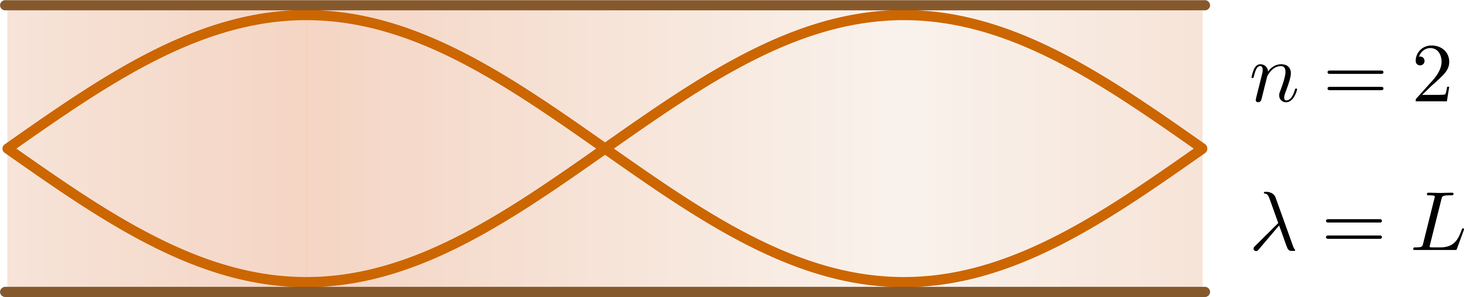
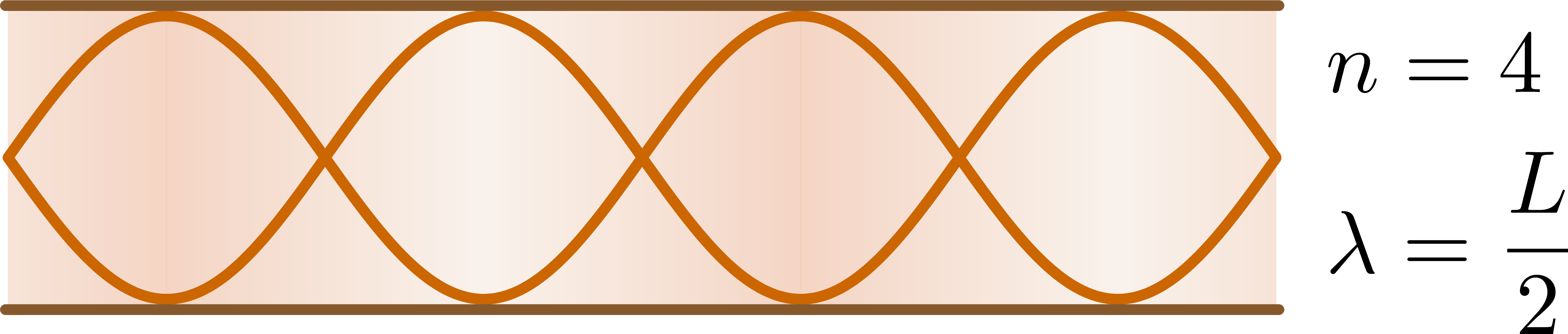
Open pipe

Edit and compile if you like:
% Author: Izaak Neutelings (December 2020)
% http://hyperphysics.phy-astr.gsu.edu/hbase/Waves/standw.html
\documentclass[border=3pt,tikz]{standalone}
\usepackage{amsmath}
\usepackage{etoolbox} % ifthen
\usepackage{tikz}
\usetikzlibrary{arrows.meta} % for arrow size
\tikzset{>=latex} % for LaTeX arrow head

\colorlet{xcol}{blue!70!black}
\colorlet{vcol}{green!60!black}
\colorlet{Pcol}{orange!80!black}
\colorlet{dense air}{Pcol!70!red!60}
\colorlet{thin air}{brown!10}
\colorlet{myred}{red!65!black}
\tikzstyle{vvec}=[->,vcol,very thick,line cap=round]
\tikzstyle{wood}=[very thick,brown!70!black]
\tikzstyle{Pline}=[Pcol,very thick,line cap=round]
\def\tick#1#2{\draw[thick] (#1) ++ (#2:0.1) --++ (#2-180:0.2)}
\tikzstyle{myarr}=[xcol!50,-{Latex[length=3,width=2]}]

\begin{document}

% STANDING WAVE
\begin{tikzpicture}
  \message{Standing wave plot...^^J}
  \def\lam{2.0}      % wavelength
  \def\n{2}          % harmonic
  \def\L{\n*\lam}    % length
  \def\ymax{0.85}    % y maximum
  \def\xmax{1.02*\L} % x maximum
  \def\A{0.80*\ymax} % amplitude
  \def\D{1.20*\ymax} % pipe diameter
  \def\s{2.45*\ymax} % shift
  \def\N{1200}       % number of points
  %\def\N{500}        % number of points

  % DISPLACEMENT
  \foreach \i [evaluate={\x=(\i-0.75)*\lam;}] in {1,...,\n}{
    \draw[myarr] (\x,0.15*\A) --++ (0,0.65*\A);
    \draw[myarr] (\x+\lam/2,-0.15*\A) --++ (0,-0.65*\A);
    \draw[blue!20!black!60,very thin,dashed] (\x+\lam/4,\ymax) --++ (0,-2.8*\s);
    \draw[blue!20!black!60,very thin,dashed] (\x+3*\lam/4,\ymax) --++ (0,-2.8*\s);
  }
  \draw[->,thick] (0,-\ymax) -- (0,0.1+\ymax) node[below=2,left] {$s$};
  \draw[->,thick] (-0.2*\ymax,0) -- (0.2+\xmax,0) node[below] {$x$};
  \draw[xcol,very thick,samples=100,smooth,variable=\x,domain=0:\L]
    plot(\x,{\A*sin(360/\lam*\x)});
  \draw[xcol,dashed,samples=100,smooth,variable=\x,domain=0:\L]
    plot(\x,{-\A*sin(360/\lam*\x)});

  % PRESSURE
  \begin{scope}[shift={(0,-\s)}]
    \draw[->,thick] (0,-\ymax) -- (0,0.1+\ymax) node[below=2,left] {$\Delta P$};
    \draw[->,thick] (-0.2*\ymax,0) -- (0.2+\xmax,0) node[below] {$x$};
    \draw[Pcol,very thick,samples=100,smooth,variable=\x,domain=0:\L]
      plot(\x,{\A*sin(360/\lam*\x-90)});
    \draw[Pcol,dashed,samples=100,smooth,variable=\x,domain=0:\L]
      plot(\x,{-\A*sin(360/\lam*\x-90)});
  \end{scope}

  % TUBE, t = 0
  \message{  Generating gas particles at t = 0...^^J}
  \begin{scope}[shift={(0,-2.1*\s)}]
    \fill[thin air] (0,0) rectangle++ (\L,\D); % to fill seams
    \foreach \i [evaluate={\x=(\i-1)*\lam;}] in {1,...,\n}{
      \draw[myarr] (\x+0.25*\lam,1.1*\D) --++ ( 0.21*\lam,0);
      \draw[myarr] (\x+0.75*\lam,1.1*\D) --++ (-0.21*\lam,0);
      \path[left color=thin air,right color=thin air,middle color=dense air]
        (\x,0) rectangle (\x+\lam,\D);
      \foreach \i in {1,...,\N}{
        \fill[blue!40!black] ({\x+acos(-rand)*\lam/180},{\D*(1+rand)/2}) circle(0.01);
      }
    }
    \draw[wood] (0,0) rectangle++ (\L,\D);
    \node[left=1,scale=0.8] at (0,\D/2) {$t=0$};
  \end{scope}

  % TUBE, t = T/2
  \message{  Generating gas particles at t = T/2...^^J}
  \begin{scope}[shift={(0,-2.8*\s)}]
    \fill[dense air] (0,0) rectangle++ (\L,\D); % to fill seams
    \foreach \i [evaluate={\x=(\i-1)*\lam;}] in {1,...,\n}{
      \draw[myarr] (\x+0.25*\lam,1.1*\D) --++ (-0.21*\lam,0);
      \draw[myarr] (\x+0.75*\lam,1.1*\D) --++ ( 0.21*\lam,0);
      \path[left color=dense air,right color=dense air,middle color=thin air]
        (\x,0) rectangle (\x+\lam,\D);
    }
    \foreach \i [evaluate={\x=(\i-2)*\lam;}] in {2,...,\n}{
      \foreach \i in {1,...,\N}{
        \fill[blue!40!black] ({\x+\lam/2+acos(-rand)*\lam/180},{\D*(1+rand)/2}) circle(0.01);
      }
    }
    \foreach \i in {1,...,\N}{
      \ifodd\i
        \fill[blue!40!black] ({acos(-(rand+1)/2)*\lam/180-\lam/2},{\D*(1+rand)/2}) circle(0.01);
      \else
        \fill[blue!40!black] ({\L+acos(-(rand-1)/2)*\lam/180-\lam/2},{\D*(1+rand)/2}) circle(0.01);
      \fi
    }
    \draw[wood] (0,0) rectangle++ (\L,\D);
    \node[left=1,scale=0.8] at (0,\D/2) {$t=T/2$};
  \end{scope}

\end{tikzpicture}


%%%%%%%%%%%%%%%%%%%%%%%%%%
% STANDING WAVE - CLOSED %
%%%%%%%%%%%%%%%%%%%%%%%%%%

% STANDING WAVE - CLOSED, n=1
\def\L{5.0} % pipe length
\def\R{0.6} % pipe radius
\def\wave#1{
  \message{Standing wave #1 (closed)..^^J}
  \pgfmathsetmacro\lam{2*\L/#1} % wavelength
  \clip (-0.1,-1.3*\R) rectangle (1.27*\L,1.1*\R); % same canvas size
  \fill[thin air] (0,-\R) rectangle (\L,\R);
  \foreach \i in {1,...,#1}{
    \path[left color=thin air,right color=dense air,
          opacity=0.3,shading angle={(2*\i+1)*90}]
      ({(\i-1)*\lam/2},-\R) rectangle++ (\lam/2,2*\R);
  }
  \draw[Pline,samples=100,smooth,variable=\x,domain=0:\L]
    plot(\x,{ (\R-0.041)*cos(360/(\lam)*\x)})
    plot(\x,{-(\R-0.041)*cos(360/(\lam)*\x)});
  \draw[wood] (-0.01,-\R) rectangle (\L+0.01,\R);
  %\draw[->,thick] (0,-1.2*\R) -- (0,0.2+1.2*\R) node[left] {$\Delta P$};
  %\draw[->,thick] (-0.2*\R,0) -- (0.2+\L,0) node[below] {$x$};
  %\path (0,-1.3*\R) rectangle (1.3*\L,1.1*\R); % same canvas size
}
\begin{tikzpicture}
  \draw[<->] (0,-1.3*\R) --++ (\L,0)
    node[midway,below=-4,fill=white,inner sep=0.5,scale=0.8] {$L=\lambda/2$};
  \wave{1}
  \node[right=2,align=left] at (\L,0) {$n=1$\\[1mm]$\lambda=2L$};
\end{tikzpicture}

% STANDING WAVE - CLOSED, n=2
\begin{tikzpicture}
  \wave{2}
  \node[right=2,align=left] at (\L,0) {$n=2$\\[1mm]$\lambda=L$};
\end{tikzpicture}

% STANDING WAVE - CLOSED, n=3
\begin{tikzpicture}
  \wave{3}
  \node[below=3,right=2,align=left] at (\L,0) {$n=3$\\[2mm]$\lambda=\dfrac{2L}{3}$};
\end{tikzpicture}

% STANDING WAVE - CLOSED, n=4
\begin{tikzpicture}
  \wave{4}
  \node[below=3,right=2,align=left] at (\L,0) {$n=4$\\[2mm]$\lambda=\dfrac{L}{2}$};
\end{tikzpicture}


%%%%%%%%%%%%%%%%%%%%%%%%%%%%%
% STANDING WAVE - HALF-OPEN %
%%%%%%%%%%%%%%%%%%%%%%%%%%%%%

% STANDING WAVE - HALF-OPEN, n=1
\def\wave#1{
  \message{Standing wave #1 (half-open)..^^J}
  \pgfmathsetmacro\lam{4*\L/(2*#1-1)} % wavelength
  \clip (-0.1,-1.3*\R) rectangle (1.27*\L,1.1*\R); % same canvas size
  \fill[thin air] (0,-\R) rectangle (\L,\R);
  \begin{scope}
    \clip (0,-\R) rectangle (\L,\R);
    \foreach \i in {1,...,#1}{
      \path[left color=thin air,right color=dense air,
            opacity=0.3,shading angle={(2*\i+1)*90}]
        ({(\i-1)*\lam/2},-\R) rectangle++ (\lam/2,2*\R);
    }
  \end{scope}
  \draw[Pline,samples=100,smooth,variable=\x,domain=0:\L]
    plot(\x,{ (\R-0.041)*cos(360/(\lam)*\x)})
    plot(\x,{-(\R-0.041)*cos(360/(\lam)*\x)});
  \draw[wood,line cap=round]
     (\L+0.01,\R) -| (-0.01,-\R) -- (\L+0.01,-\R);
  %\draw[->,thick] (0,-1.2*\R) -- (0,0.2+1.2*\R) node[left] {$\Delta P$};
  %\draw[->,thick] (-0.2*\R,0) -- (0.2+\L,0) node[below] {$x$};
}
\begin{tikzpicture}
  \draw[<->] (0,-1.3*\R) --++ (\L,0)
    node[midway,below=-4,fill=white,inner sep=0.5,scale=0.8] {$L=\lambda/4$};
  \wave{1}
  \node[right=2,align=left] at (\L,0) {$n=1$\\[1mm]$\lambda=4L$};
\end{tikzpicture}

% STANDING WAVE - HALF-OPEN, n=3
\begin{tikzpicture}
  \wave{2}
  \node[below=3,right=2,align=left] at (\L,0) {$n=3$\\[2mm]$\lambda=\dfrac{4L}{3}$};
\end{tikzpicture}

% STANDING WAVE - HALF-OPEN, n=5
\begin{tikzpicture}
  \wave{3}
  \node[below=3,right=2,align=left] at (\L,0) {$n=5$\\[2mm]$\lambda=\dfrac{4L}{5}$};
\end{tikzpicture}

% STANDING WAVE - HALF-OPEN, n=7
\begin{tikzpicture}
  \wave{4}
  \node[below=3,right=2,align=left] at (\L,0) {$n=7$\\[2mm]$\lambda=\dfrac{4L}{7}$};
\end{tikzpicture}


%%%%%%%%%%%%%%%%%%%%%%%%%%%%%
% STANDING WAVE - OPEN-OPEN %
%%%%%%%%%%%%%%%%%%%%%%%%%%%%%

% STANDING WAVE - OPEN-OPEN, n=1
\def\wave#1{
  \message{Standing wave #1 (open-open)..^^J}
  \pgfmathsetmacro\lam{2*\L/#1} % wavelength
  \clip (-0.1,-1.3*\R) rectangle (1.27*\L,1.1*\R); % same canvas size
  \fill[thin air] (0,-\R) rectangle (\L,\R);
  \begin{scope}
    \clip (0,-\R) rectangle (\L,\R);
    \foreach \i in {0,...,#1}{
      \path[left color=thin air,right color=dense air,
            opacity=0.3,shading angle={(2*\i+1)*90}]
        ({(\i-0.5)*\lam/2},-\R) rectangle++ (\lam/2,2*\R);
    }
  \end{scope}
  \draw[Pline,samples=100,smooth,variable=\x,domain=0:\L]
    plot(\x,{ (\R-0.041)*sin(360/(\lam)*\x)})
    plot(\x,{-(\R-0.041)*sin(360/(\lam)*\x)});
  \draw[wood,line cap=round]
    (-0.01, \R) -- (\L+0.01, \R)
    (-0.01,-\R) -- (\L+0.01,-\R);
  %\draw[->,thick] (0,-1.2*\R) -- (0,0.2+1.2*\R) node[left] {$\Delta P$};
  %\draw[->,thick] (-0.2*\R,0) -- (0.2+\L,0) node[below] {$x$};
}
\begin{tikzpicture}
  \draw[<->] (0,-1.3*\R) --++ (\L,0)
    node[midway,below=-4,fill=white,inner sep=0.5,scale=0.8] {$L=\lambda/2$};
  \wave{1}
  \node[right=2,align=left] at (\L,0) {$n=1$\\[1mm]$\lambda=2L$};
\end{tikzpicture}

% STANDING WAVE - OPEN-OPEN, n=2
\begin{tikzpicture}
  \wave{2}
  \node[right=2,align=left] at (\L,0) {$n=2$\\[2mm]$\lambda=L$};
\end{tikzpicture}

% STANDING WAVE - OPEN-OPEN, n=3
\begin{tikzpicture}
  \wave{3}
  \node[below=3,right=2,align=left] at (\L,0) {$n=3$\\[2mm]$\lambda=\dfrac{2L}{3}$};
\end{tikzpicture}

% STANDING WAVE - OPEN-OPEN, n=4
\begin{tikzpicture}
  \wave{4}
  \node[below=3,right=2,align=left] at (\L,0) {$n=4$\\[2mm]$\lambda=\dfrac{L}{2}$};
\end{tikzpicture}

\end{document}
Click to download: waves_standing_air.tex • waves_standing_air.pdf
Open in Overleaf: waves_standing_air.tex


Hello Izaak,
Let me ask you something (not tikz related), in the first diagram of this series, I see that the arrows on the “tubes” t=0 and t = T/2 are always pointing from low to high pressure. Could explain why that is?
I just thought that pointing from high to low pressure would be the “correct” way.
Thank you,
Wagner.
Hi Wagner,
It is to indicate movement, or equivalently, the displacement (s) of air molecules which is 90° out of phase with pressure differences (ΔP), which is why I used blue arrows, like the blue graph of s vs. time. I guess it could be made more explicit and clear by indicating an “s” above the arrows.
Izaak
Nodes and anti nodes are exchanged, right? Open pipes should have anti nodes at their ends, closed ones should have nodes at their ends, but here it’s the opposite? Is it a mistake or am I missing anything?
Thank you very much for these resources.
Hi Rodrigo,
Are you talking about amplitude of the displacement s, the blue line in the first figure), or the amplitude of the pressure difference ΔP, shown as by the orange lines? They are 90° out of phase, as shown in the first figure, but I think the nodes are correct if they indicate those of the amplitude of pressure difference, because the pressure at an open end equalizes with the outside/atmosphere, right?
You can have a look at a more in depth discussion here (archived).
Cheers,
Izaak
Oh, now I understand. Those lines are representing pressure differences. It’s just that I’m more used to see them representing wave amplitudes (actual displacement of the particles), especially when comparing waves on a string and waves in pipes. I just edited the figures, basically changing sin to cos. Again, thank you very much for these resources. I’m using them extensively, properly referencing the source (I typically translate them or modify fonts/notation, which is super easy thanks to having the .tex source).