Merit zT vs. carrier concentration n

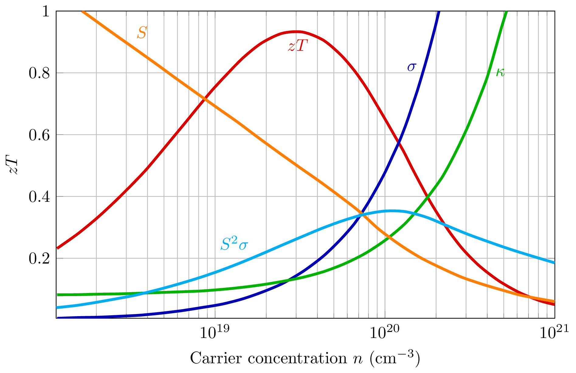
Thermoelectric figure of merit $zT$ vs carrier concentration $n$ for \ch{Bi2Te3} based on empirical data in ref.~\cite{rowe_alpha-sigma_1995}. Tuning $n$ for optimal $zT$ involves a compromise between thermal conductivity $\kappa$, Seebeck coefficient $S$ and electrical conductivity $\sigma$.
Increasing the electrical conductivity $\sigma$ not only produces an increase in the electronic thermal conductivity $\kappa_\text{el}$ but also usually decreases the Seebeck coefficient $S$. This makes optimal $\zT$ difficult to achieve. Plot scales are $\kappa/\si{\watt\per\meter\per\kelvin} \in [0,10]$, $S/\si{\micro\volt\per\kelvin} \in [0,500]$, $\sigma/\si{\per\ohm\per\centi\meter} \in [0,5000]$.

Edit and compile if you like:

1
2
3
4
5
6
7
8
9
10
11
12
13
14
15
16
17
18
19
20
21
22
23
24
25
26
27
28
29
30
31
32
33
34
35
36
37
38
39
40
41
% Thermoelectric figure of merit $zT$ vs carrier concentration $n$ for \ch{Bi2Te3} based on empirical data in ref.~\cite{rowe_alpha-sigma_1995}. Tuning $n$ for optimal $zT$ involves a compromise between thermal conductivity $\kappa$, Seebeck coefficient $S$ and electrical conductivity $\sigma$. Increasing the electrical conductivity $\sigma$ not only produces an increase in the electronic thermal conductivity $\kappa_\text{el}$ but also usually decreases the Seebeck coefficient $S$. This makes optimal $\zT$ difficult to achieve. Plot scales are $\kappa/\si{\watt\per\meter\per\kelvin} \in [0,10]$, $S/\si{\micro\volt\per\kelvin} \in [0,500]$, $\sigma/\si{\per\ohm\per\centi\meter} \in [0,5000]$.
\documentclass[tikz]{standalone}
\usepackage{pgfplots,siunitx}
\pgfplotsset{compat=newest}
\begin{document}
\begin{tikzpicture}
  \begin{axis}[
      xmode=log,
      domain=1e17:1e21,
      ymax=1,
      enlargelimits=false,
      ylabel=$zT$,
      xlabel=Carrier concentration $n$ (\si{\per\centi\meter\cubed}),
      grid=both,
      width=12cm,
      height=8cm,
      decoration={name=none},
    ]
    \addplot [ultra thick, smooth, red!85!black] coordinates {
        (1.174e+18, 0.2317)
        (1.551e+18, 0.2787)
        (2.016e+18, 0.3300)
        (2.549e+18, 0.3816)
        (3.171e+18, 0.4332)
        (3.891e+18, 0.4842)
        (4.697e+18, 0.5373)
        (5.623e+18, 0.5892)
        (6.714e+18, 0.6404)
        (8.017e+18, 0.6923)
        (9.650e+18, 0.7450)
        (1.178e+19, 0.7963)
        (1.461e+19, 0.8486)
        (1.878e+19, 0.8964)
        (2.481e+19, 0.9278)
        (3.279e+19, 0.9318)
        (4.334e+19, 0.9057)
        (5.515e+19, 0.8571)
 
 
הההההההההההההההההההההההההההההההההההההההההההההההההההההההההההההההההההההההההההההההההההההההההההההההההההההההההההההההההההההההההההההההההההההההההההההההההההההההההההההההההההההההההההההההההההההההההההההההההההההההההההההההההההההההההההההההההההההההההההההההההההההההההההההההה
XXXXXXXXXXXXXXXXXXXXXXXXXXXXXXXXXXXXXXXXXXXXXXXXXXXXXXXXXXXXXXXXXXXXXXXXXXXXXXXXXXXXXXXXXXXXXXXXXXXXXXXXXXXXXXXXXXXXXXXXXXXXXXXXXXXXXXXXXXXXXXXXXXXXXXXXXXXXXXXXXXXXXXXXXXXXXXXXXXXXXXXXXXXXXXXXXXXXXXXXXXXXXXXXXXXXXXXXXXXXXXXXXXXXXXXXXXXXXXXXXXXXXXXXXXXXXXXX