")


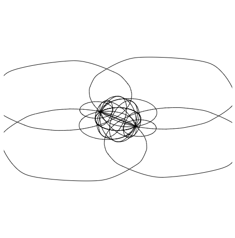
If you take the stereographic projection of a mesh sphere, you obtain Steiner circles.
Interestingly, the map of any inscribed circle of the sphere under stereographic projection is a perfect circle on the plane.
Unfortunately, due to the low sampling size, the smooth option can be a bit botched sometimes.
The code is parameterized so that the user can specify Euler angle rotations of the sphere, and see the resulting stereographic projection on the plane.
If a line goes near the north pole, we omit it by setting the opacity to zero.
There are other workarounds, but they require using a conditional in a for loop, and I wanted to use the smooth option.
For example, this animation shows the sphere undergoing a rotation which is based on all three angles changing differently:
Try changing the values of \zrotationa, \yrotation and \zrotationb for yourself!
\documentclass[
    tikz
    ,border = 3.14mm
]{standalone}
\usepackage{tikz-3dplot}
\pgfmathdeclarefunction{sphereX}{2}{%
    % #1  - longitude
    % #2  - latitude
    \pgfmathparse{cos(#2)*cos(#1)}%
}
\pgfmathdeclarefunction{sphereY}{2}{%
    \pgfmathparse{cos(#2)*sin(#1)}%
}
\pgfmathdeclarefunction{sphereZ}{2}{%
    \pgfmathparse{sin(#2)}%
}
% https://tex.stackexchange.com/a/736767/319072
\pgfmathdeclarefunction{tdplottransformrotmainX}{6}{%
    % #1  - Z rotation
    % #2  - Y rotation
    % #3  - Z rotation
    % #4  - x value
    % #5  - y value
    % #6  - z value
    \pgfmathparse{
        (
            (
                sin(#1) * cos(#2) * cos(#3) +
                cos(#1) * sin(#3)
            ) * #4 +
            (
                -sin(#1) * cos(#2) * sin(#3) +
                cos(#1) * cos(#3)
            ) * #5 +
            sin(#1) * sin(#2) * #6
        ) * -1
    }%
}
\pgfmathdeclarefunction{tdplottransformrotmainY}{6}{%
    \pgfmathparse{
        (
            cos(#1) * cos(#2) * cos(#3) -
            sin(#1) * sin(#3)
        ) * #4 +
        (
            -cos(#1) * cos(#2) * sin(#3) -
            sin(#1) * cos(#3)
        ) * #5 +
        cos(#1) * sin(#2) * #6
    }%
}
\pgfmathdeclarefunction{tdplottransformrotmainZ}{6}{%
    \pgfmathsetmacro\tdplottransformrotmainZtemp{
        -sin(#2) * cos(#3) * #4 +
        sin(#2) * sin(#3) * #5 +
        cos(#2) * #6
    }%
    \pgfmathparse{%
        \tdplottransformrotmainZtemp > 0.995%
    }%
    \ifnum\pgfmathresult=1%
        \xdef\opacity{0}%
    \fi%
    \let\pgfmathresult\tdplottransformrotmainZtemp%
}
\pgfmathdeclarefunction{stereographicprojection}{2}{%
    % #1  - the x or y value of the input
    % #2  - the z value of the input
    % Returns the x or y value of the output
    \pgfmathparse{#2 < 0.995}%
    \ifnum\pgfmathresult=1%
        \pgfmathparse{#1 / (1 - #2)}%
    \else%
        \pgfmathparse{#1 / (1 - 0.995)}%
    \fi%
}
\pgfmathsetmacro{\azimuth}{130}   % viewing azimuth
\pgfmathsetmacro{\elevation}{30}  % viewing elevation
\pgfmathsetmacro{\zrotationa}{0}  % Z1 rotation of sphere
\pgfmathsetmacro{\yrotation}{90}  % Y rotation of sphere
\pgfmathsetmacro{\zrotationb}{0}  % Z2 rotation of sphere
\begin{document}
    \tdplotsetmaincoords{90-\elevation}{\azimuth}
    \begin{tikzpicture}[tdplot_main_coords]
        \clip[tdplot_screen_coords] (-5,-5) rectangle (5,5);
        \pgfmathsetmacro{\startlongitude}{-90}
        \pgfmathsetmacro{\endlongitude}{90}
        \pgfmathsetmacro{\sampleslongitude}{5}
        \pgfmathsetmacro{\steplongitude}{
            (\endlongitude - \startlongitude) /
            \sampleslongitude
        }
        \foreach \longitude[parse = true] in {%
            \startlongitude%
            ,\startlongitude + \steplongitude%
            ,...%
            ,\endlongitude%
        } {
            \xdef\opacity{1}
            \draw[
                smooth
                ,domain = 0:360
                ,samples = 35
                ,variable = \latitude
            ] plot (
                {
                    tdplottransformrotmainX(
                        \zrotationa,\yrotation,\zrotationb
                        ,sphereX(\longitude,\latitude)
                        ,sphereY(\longitude,\latitude)
                        ,sphereZ(\longitude,\latitude)
                    )
                }
                ,{
                    tdplottransformrotmainY(
                        \zrotationa,\yrotation,\zrotationb
                        ,sphereX(\longitude,\latitude)
                        ,sphereY(\longitude,\latitude)
                        ,sphereZ(\longitude,\latitude)
                    )
                }
                ,{
                    tdplottransformrotmainZ(
                        \zrotationa,\yrotation,\zrotationb
                        ,sphereX(\longitude,\latitude)
                        ,sphereY(\longitude,\latitude)
                        ,sphereZ(\longitude,\latitude)
                    )
                }
            );
            \draw[
                smooth
                ,domain = 0:360
                ,samples = 35
                ,variable = \latitude
                ,opacity = \opacity
            ] plot (
                {
                    stereographicprojection(
                        tdplottransformrotmainX(
                            \zrotationa,\yrotation,\zrotationb
                            ,sphereX(\longitude,\latitude)
                            ,sphereY(\longitude,\latitude)
                            ,sphereZ(\longitude,\latitude)
                        )
                        ,tdplottransformrotmainZ(
                            \zrotationa,\yrotation,\zrotationb
                            ,sphereX(\longitude,\latitude)
                            ,sphereY(\longitude,\latitude)
                            ,sphereZ(\longitude,\latitude)
                        )
                    )
                }
                ,{
                    stereographicprojection(
                        tdplottransformrotmainY(
                            \zrotationa,\yrotation,\zrotationb
                            ,sphereX(\longitude,\latitude)
                            ,sphereY(\longitude,\latitude)
                            ,sphereZ(\longitude,\latitude)
                        )
                        ,tdplottransformrotmainZ(
                            \zrotationa,\yrotation,\zrotationb
                            ,sphereX(\longitude,\latitude)
                            ,sphereY(\longitude,\latitude)
                            ,sphereZ(\longitude,\latitude)
                        )
                    )
                }
            );
            % Going forward, we interchange latitude and longitude to
            % find orthogonal trajectories on the sphere and on the plane.
            \xdef\opacity{1}
            \draw[
                smooth
                ,domain = 0:360
                ,samples = 35
                ,variable = \latitude
            ] plot (
                {
                    tdplottransformrotmainX(
                        \zrotationa,\yrotation,\zrotationb
                        ,sphereX(\latitude,\longitude)
                        ,sphereY(\latitude,\longitude)
                        ,sphereZ(\latitude,\longitude)
                    )
                }
                ,{
                    tdplottransformrotmainY(
                        \zrotationa,\yrotation,\zrotationb
                        ,sphereX(\latitude,\longitude)
                        ,sphereY(\latitude,\longitude)
                        ,sphereZ(\latitude,\longitude)
                    )
                }
                ,{
                    tdplottransformrotmainZ(
                        \zrotationa,\yrotation,\zrotationb
                        ,sphereX(\latitude,\longitude)
                        ,sphereY(\latitude,\longitude)
                        ,sphereZ(\latitude,\longitude)
                    )
                }
            );
            \draw[
                smooth
                ,domain = 0:360
                ,samples = 35
                ,variable = \latitude
                ,opacity = \opacity
            ] plot (
                {
                    stereographicprojection(
                        tdplottransformrotmainX(
                            \zrotationa,\yrotation,\zrotationb
                            ,sphereX(\latitude,\longitude)
                            ,sphereY(\latitude,\longitude)
                            ,sphereZ(\latitude,\longitude)
                        )
                        ,tdplottransformrotmainZ(
                            \zrotationa,\yrotation,\zrotationb
                            ,sphereX(\latitude,\longitude)
                            ,sphereY(\latitude,\longitude)
                            ,sphereZ(\latitude,\longitude)
                        )
                    )
                }
                ,{
                    stereographicprojection(
                        tdplottransformrotmainY(
                            \zrotationa,\yrotation,\zrotationb
                            ,sphereX(\latitude,\longitude)
                            ,sphereY(\latitude,\longitude)
                            ,sphereZ(\latitude,\longitude)
                        )
                        ,tdplottransformrotmainZ(
                            \zrotationa,\yrotation,\zrotationb
                            ,sphereX(\latitude,\longitude)
                            ,sphereY(\latitude,\longitude)
                            ,sphereZ(\latitude,\longitude)
                        )
                    )
                }
            );
        }
    \end{tikzpicture}
\end{document}