")


Pseudorapidity on a 2D coordinate axis. For the coordinate system of the CMS detecter at the LHC, please see this post.

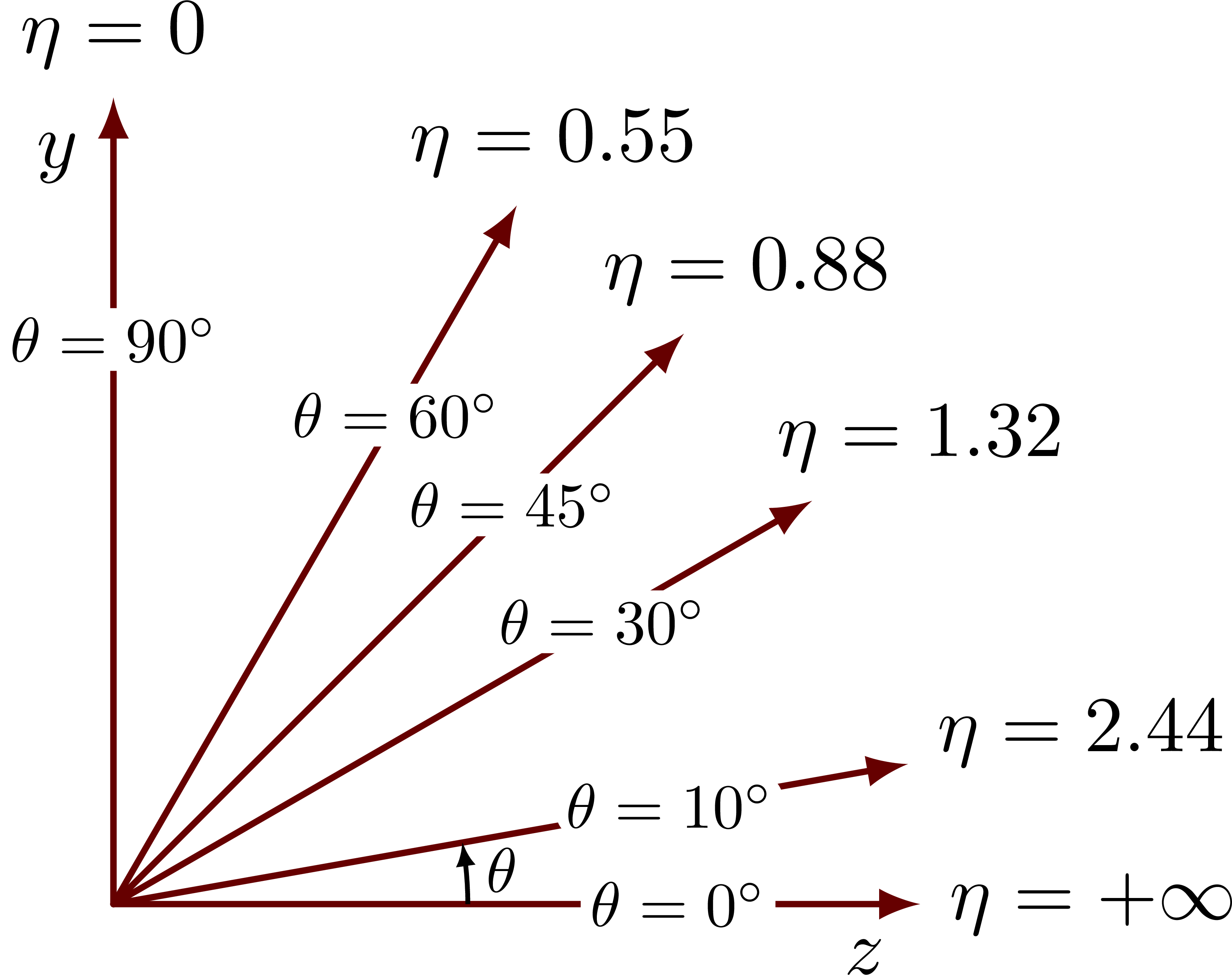
This is the simplest method with a for-loop in two variables: θ and η:
\documentclass[border=3pt,tikz]{standalone}
\tikzset{>=latex} % for LaTeX arrow head
\begin{document}
\begin{tikzpicture}[scale=3]
  \foreach \t/\e in {90/0,60/0.55,45/0.88,30/1.32,10/2.43,0/+\infty}{
    \pgfkeys{/pgf/number format/precision=2}
    \draw[->,thick] % eta lines
      (0,0) -- (\t:1.2) node[anchor=180+\t,black] {$\eta=\e$}
      node[black,pos=0.72,fill=white,scale=0.8,inner sep=2] {$\theta=\t^\circ$};
  }
\end{tikzpicture}
\end{document}
In the following method, η is calculated and rounded to two significant digits on the fly, with the exception for θ = 0:
\documentclass[border=3pt,tikz]{standalone}
\tikzset{>=latex} % for LaTeX arrow head
\usetikzlibrary{fpu} % for higher floating-point precision
\pgfkeys{
  /pgf/fpu/output format=fixed, % fpu floating-point format
  /pgf/number format/precision=2 % two decimals
}
\begin{document}
\begin{tikzpicture}[scale=3]
  \foreach \t in {90,60,45,30,10,0}{
    \ifnum \t = 0
      \def\e{+\infty} % infinity symbol
    \else
      \pgfkeys{/pgf/fpu=true} % increase floating-point precision in computation
      \pgfmathparse{-ln(tan(\t/2))} % pseudorapidity
      \pgfkeys{/pgf/fpu=false} % turn off to avoid interference with following
      \pgfmathroundtozerofill{\pgfmathresult} % round with trailing zeroes
      \pgfmathsetmacro\e{\t==90?0:\pgfmathresult} % no trailing zeroes for theta = 0
    \fi
    \draw[->,thick] % eta lines
      (0,0) -- (\t:1.2) node[anchor=180+\t,black] {$\eta=\e$}
      node[black,pos=0.72,fill=white,scale=0.8,inner sep=2] {$\theta=\t^\circ$};
  }
\end{tikzpicture}
\end{document}
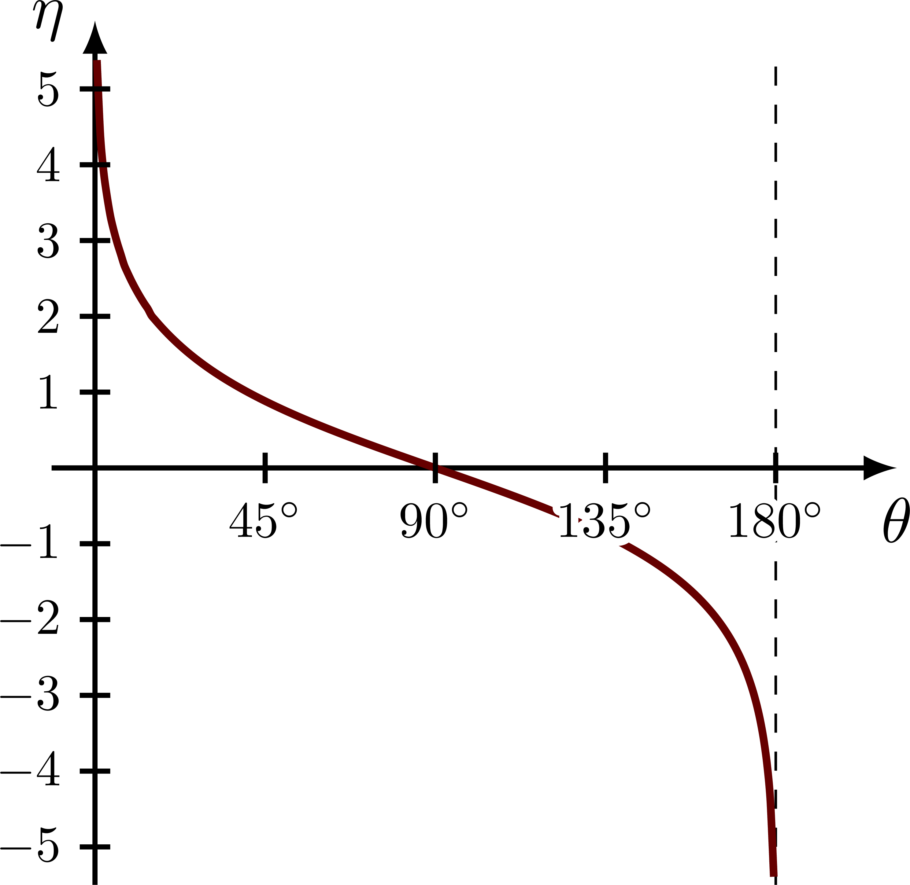
The fpu package was needed to increase the precision of the pseudorapidity η = -ln(tan(θ/2)) computation; otherwise, there would be an O(1%) error because the default PGF math engine uses limited-precision fixed-point arithmetic with roughly 5–6 decimal digits.
Full code
Edit and compile if you like:
% Author: Izaak Neutelings (June 2017)
% Updated: December 2022, March 2026
\documentclass[border=3pt,tikz]{standalone}
\usepackage[outline]{contour} % glow around text
\usetikzlibrary{angles,quotes} % for pic (angle labels)
\usetikzlibrary{arrows.meta} % for arrow head size
\usetikzlibrary{bending} % for bending arrow head
\usetikzlibrary{fpu} % for higher floating-point precision
\contourlength{1.5pt}
% TIKZ STYLES
\tikzset{
>=latex, % for LaTeX arrow head
eta line/.style={->,black!60!red,thick,line cap=round},
theta node/.style={black,pos=0.7,fill=white,scale=0.8,
inner sep=1.5pt,rounded corners=3pt},
mysmallarrow/.style={-{Latex[length=3,width=2.5]},draw=black,line width=0.6,
angle radius=45,angle eccentricity=1.1}
}
\begin{document}
% PSEUDORAPIDITY with manual for-loop over theta, eta
\begin{tikzpicture}[scale=3]
\message{^^JPseudorapidity simple}
\def\R{1.2} % radius/length of lines
\node[scale=1,below left=1] at (0,\R) {$y$}; % y axis
\node[scale=1,below left=1] at (\R,0) {$z$}; % z axis
\foreach \t/\e in {90/0,60/0.55,45/0.88,30/1.32,10/2.44,0/+\infty}{ % loop over theta/eta
\pgfkeys{/pgf/number format/precision=2}
\draw[eta line] % eta lines
(0,0) -- (\t:\R) node[anchor=180+\t,black] {$\eta=\e$}
node[theta node] {$\theta=\t^\circ$};
}
%\draw[black!60!red,thick] (0,0.1*\R) |- (0.1*\R,0) ; % overlap in corner
\end{tikzpicture}
% PSEUDORAPIDITY with automatic calculation of eta
\begin{tikzpicture}[scale=3]
\message{^^JPseudorapidity with automatic calculation of eta}
\pgfkeys{
/pgf/fpu/output format=fixed, % fpu floating-point format
/pgf/number format/precision=2 % two decimals
}
\def\R{1.2} % radius/length of lines
\node[scale=1,below left=1] at (0,\R) {$y$}; % y axis
\node[scale=1,below left=1] at (\R,0) {$z$}; % z axis
\coordinate (O) at (0,0); % origin
\foreach \t in {90,60,45,30,10,0}{ % loop over theta
\ifnum \t = 0
\def\e{+\infty} % infinity symbol
\else
\pgfkeys{/pgf/fpu=true} % increase floating-point precision in computation
\pgfmathparse{-ln(tan(\t/2))} % pseudorapidity
\pgfkeys{/pgf/fpu=false} % turn off to avoid interference with following
\pgfmathroundtozerofill{\pgfmathresult} % round with trailing zeroes
\pgfmathsetmacro\e{\t==90?0:\pgfmathresult} % no trailing zeroes for theta = 0
\fi
\message{^^Jt=\t, e=\e}
\draw[eta line] % eta lines
(O) -- (\t:\R) coordinate(P\t) node[anchor=180+\t,black] {$\eta=\e$}
node[theta node] {$\theta=\t^\circ$};
}
%\draw[black!60!red,thick] (0,0.1*\R) |- (0.1*\R,0) ; % overlap in corner
\draw pic["$\theta$"scale=0.8,mysmallarrow] {angle = P0--O--P10}; % arrow label
\end{tikzpicture}
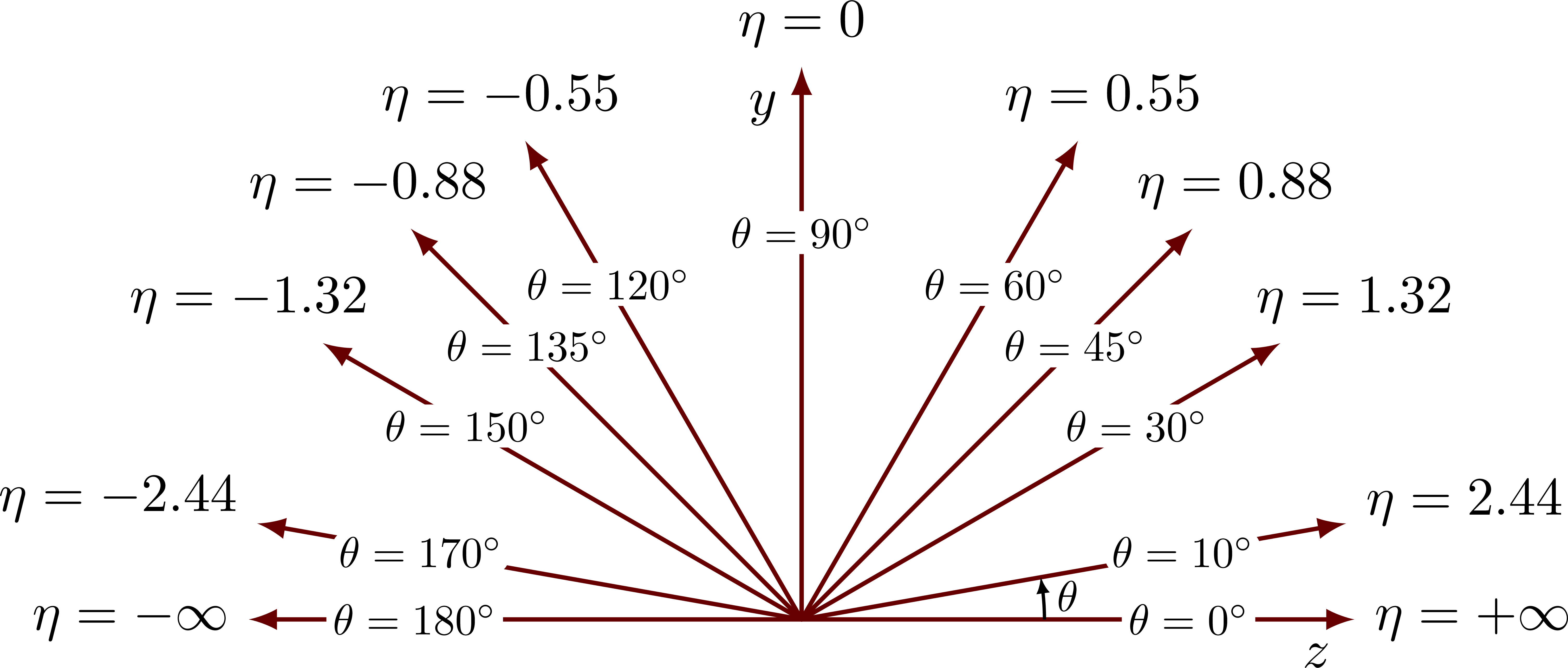
% PSEUDORAPIDITY including negative side
\begin{tikzpicture}[scale=3]
\message{^^JPseudorapidity including negative side}
\pgfkeys{
/pgf/fpu/output format=fixed, % fpu floating-point format
/pgf/number format/precision=2 % two decimals
}
\def\R{1.2} % radius/length of lines
\node[scale=1,below left=1] at (0,\R) {$y$}; % y axis
\node[scale=1,below left=1] at (\R,0) {$z$}; % z axis
\foreach \t in {180,170,150,135,120,90,60,45,30,10,0}{ % loop over theta
\ifnum \t = 0
\def\e{+\infty} % infinity symbol
\else \ifnum \t = 180
\def\e{-\infty} % infinity symbol
\else
\pgfkeys{/pgf/fpu=true} % increase floating-point precision in computation
\pgfmathparse{-ln(tan(\t/2))} % pseudorapidity
\pgfkeys{/pgf/fpu=false} % turn off to avoid interference with following
\pgfmathroundtozerofill{\pgfmathresult} % round with trailing zeroes
\pgfmathsetmacro\e{\t==90?0:\pgfmathresult} % no trailing zeroes for theta = 0
\fi \fi
\message{^^Jt=\t, e=\e}
\draw[eta line] % eta lines
(0,0) -- (\t:\R) coordinate(P\t) node[anchor=180+\t,black] {$\eta=\e$}
node[theta node] {$\theta=\t^\circ$};
}
\draw pic["$\theta$"scale=0.8,mysmallarrow] {angle = P0--O--P10}; % arrow label
\end{tikzpicture}
% PSEUDORAPIDITY: plot eta vs. theta
\begin{tikzpicture}[scale=1.2,x=1cm,y=0.35cm,tick/.style={thick,scale=0.8}]
% SETTINGS
\def\ltick{2pt} % length of ticks
\def\xmax{3.7} % maximum x (theta)
\def\ymax{5.5} % maximum y (eta)
\pgfmathsetmacro\tmax{2*atan(exp(-0.98*\ymax))} % maximum theta
\message{^^J ymax = \ymax => tmax = \tmax}
% AXIS
\draw[->,thick] (0,-\ymax) -- (0,\ymax+0.4) % y axis
node[left=1] {$\eta$};
\draw[->,thick] (-0.2,0) -- (\xmax,0) % x axis
node[below=1] {$\theta$};
\draw[dashed] (pi,-\ymax) --++ (0,2*\ymax); % asymptote
% PLOT
\draw[very thick,black!60!red,samples=200,smooth,variable=\t,domain={\tmax:180-\tmax}]
plot({rad(\t)},{-ln(tan(\t/2))});
% TICKS
\foreach \t in {45,90,...,180}{ % loop over theta
\draw[thick] ({rad(\t)},\ltick) --++ (0,-2*\ltick) % x tick
node[tick,below] {\contour{white}{$\t^\circ$}};
}
\foreach \e in {1,...,5}{ % loop over eta
\draw[thick] (\ltick,\e) --++ (-2*\ltick,0) % y tick
node[tick,left] {$\e$};
\draw[thick] (\ltick,-\e) --++ (-2*\ltick,0) % y tick
node[tick,left] {$-\e$};
}
\end{tikzpicture}
\end{document}Click to download: axis2D_pseudorapidity.tex • axis2D_pseudorapidity.pdf
Open in Overleaf: axis2D_pseudorapidity.tex


 production")