")


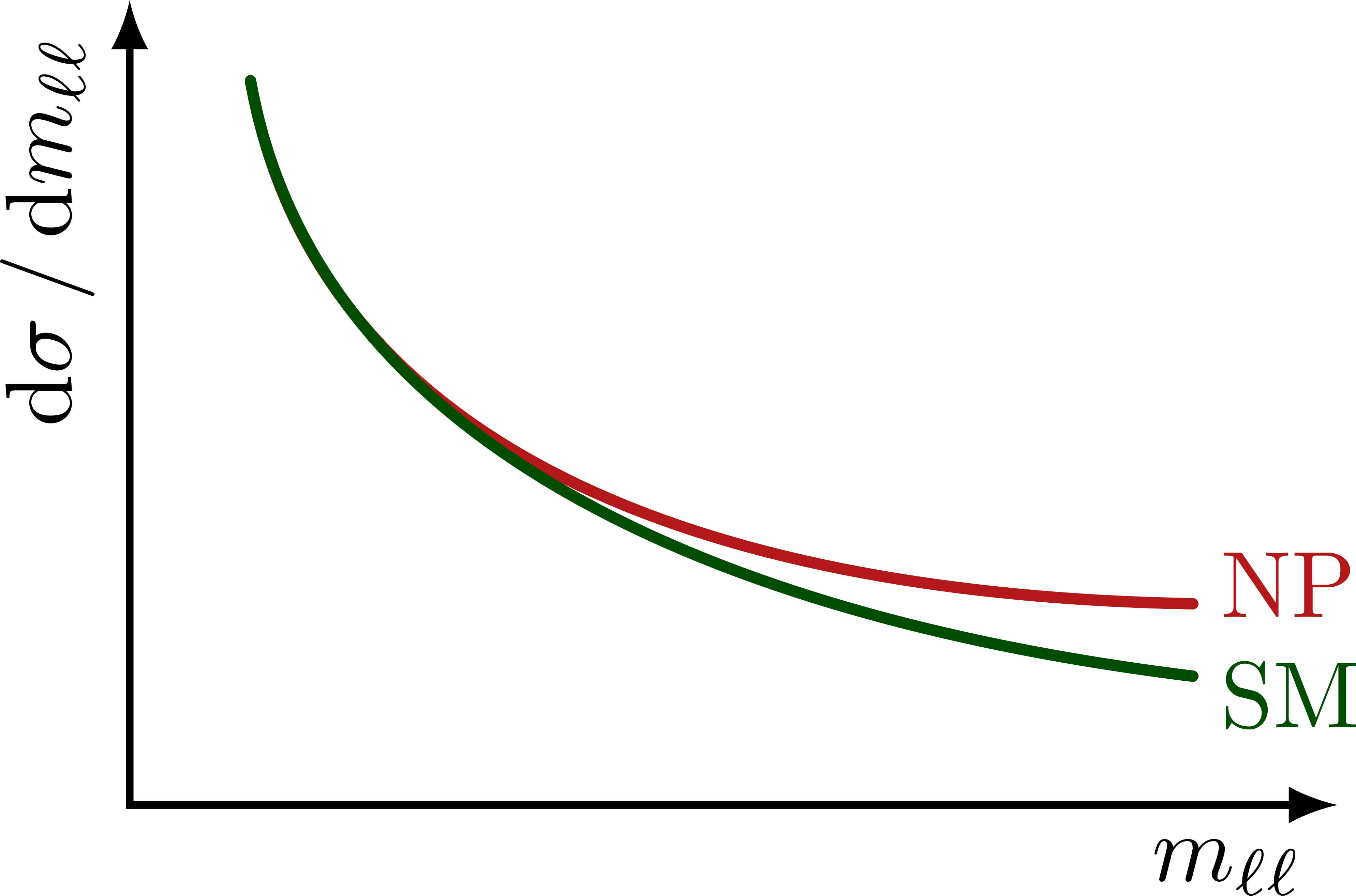
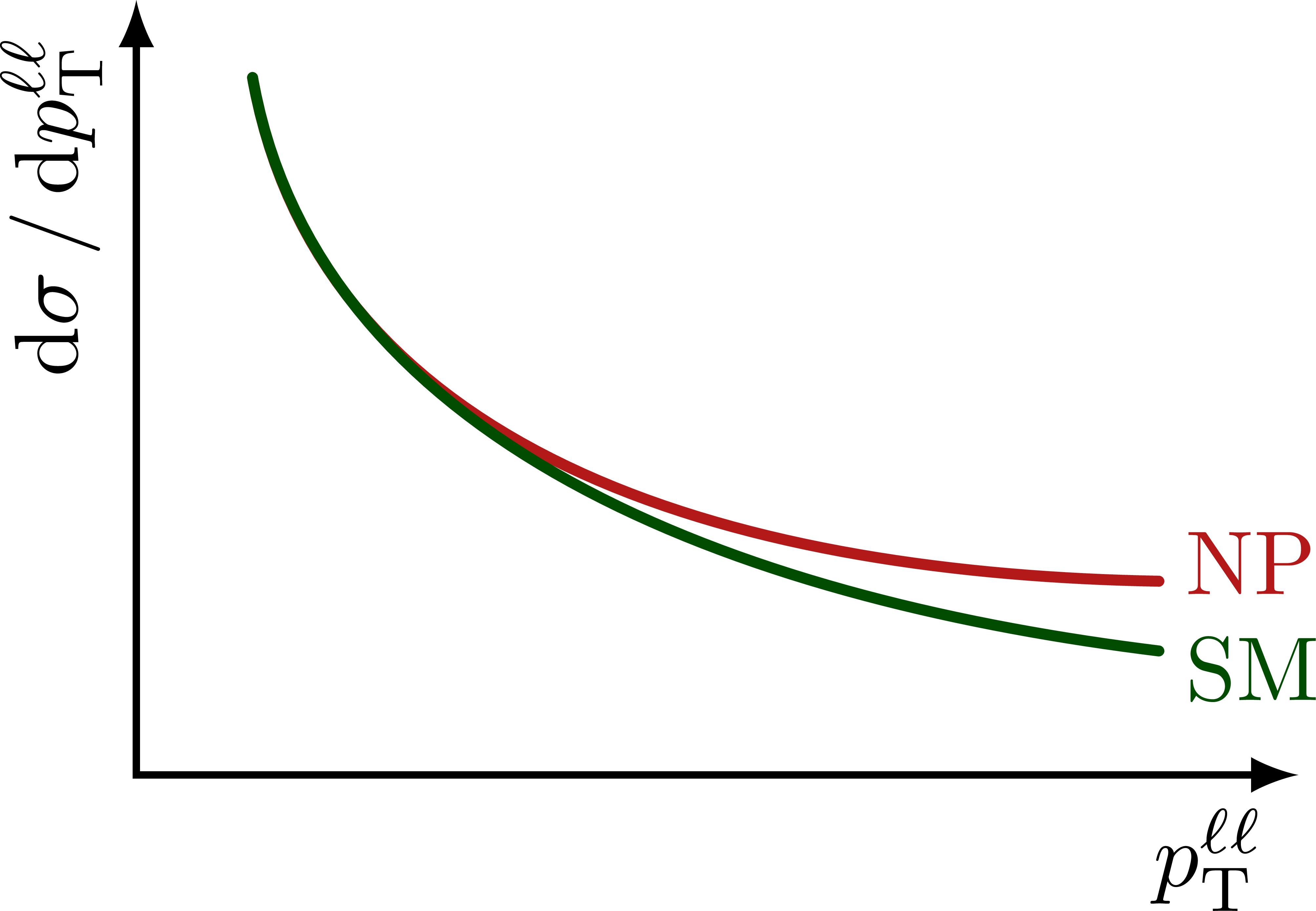
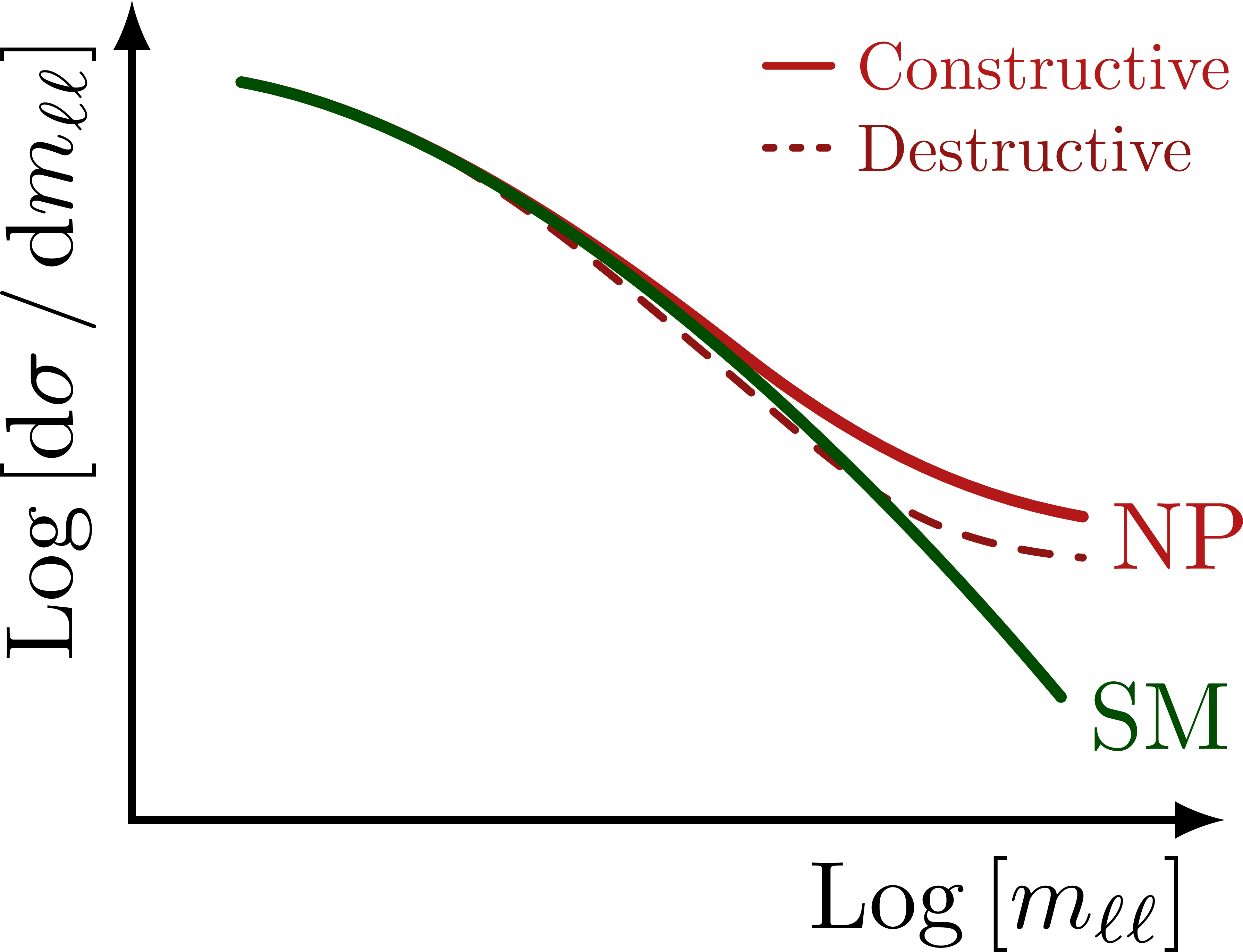
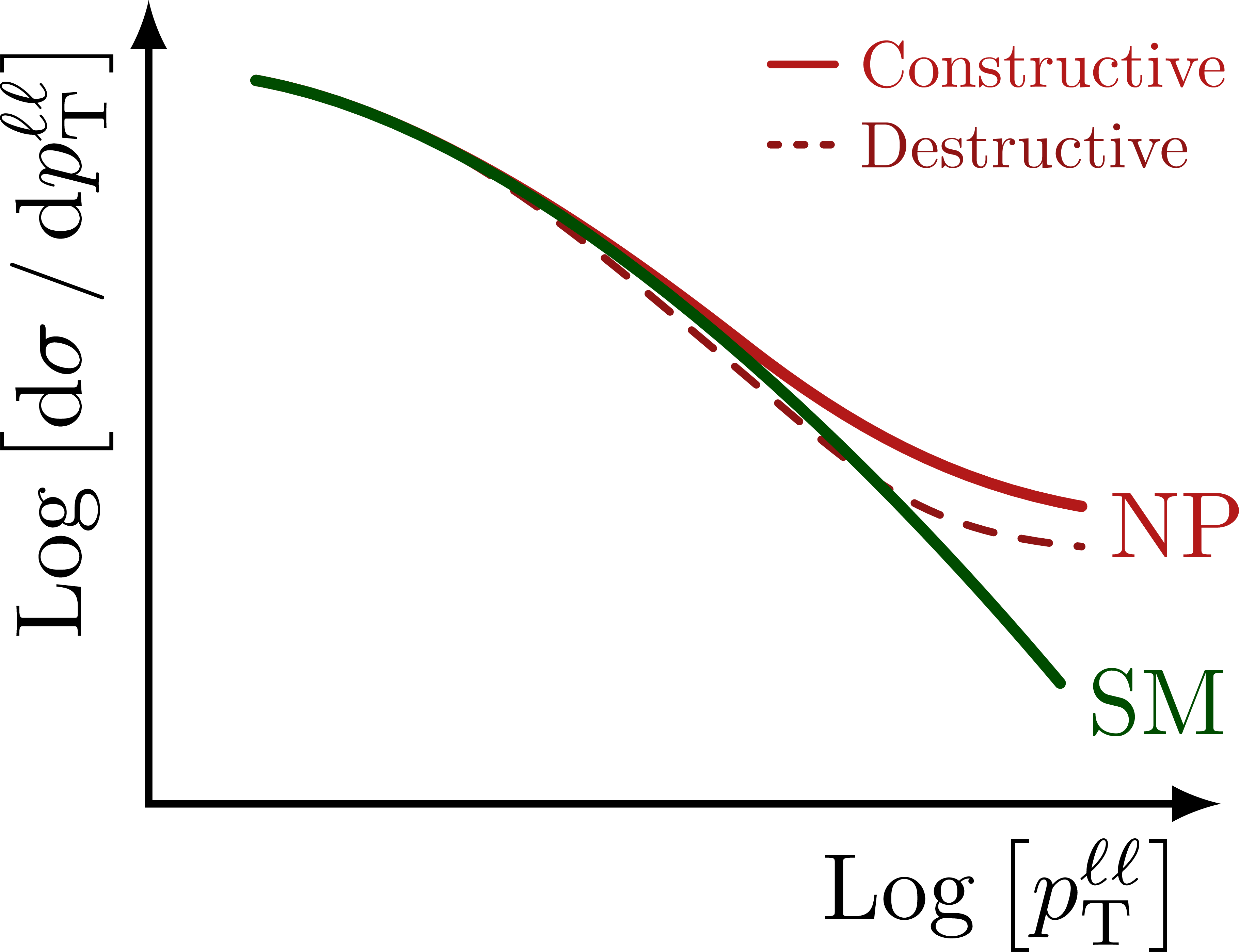
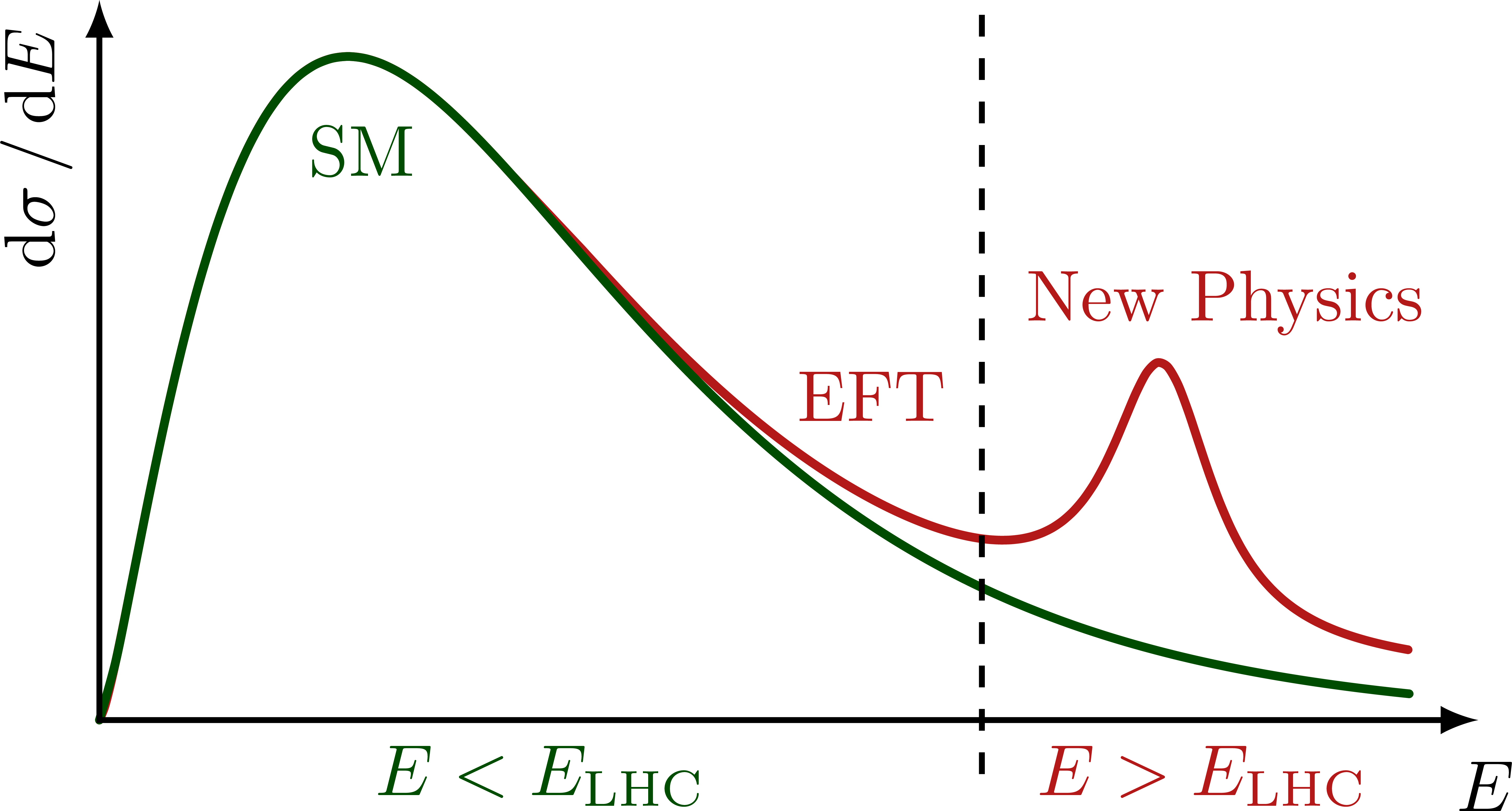
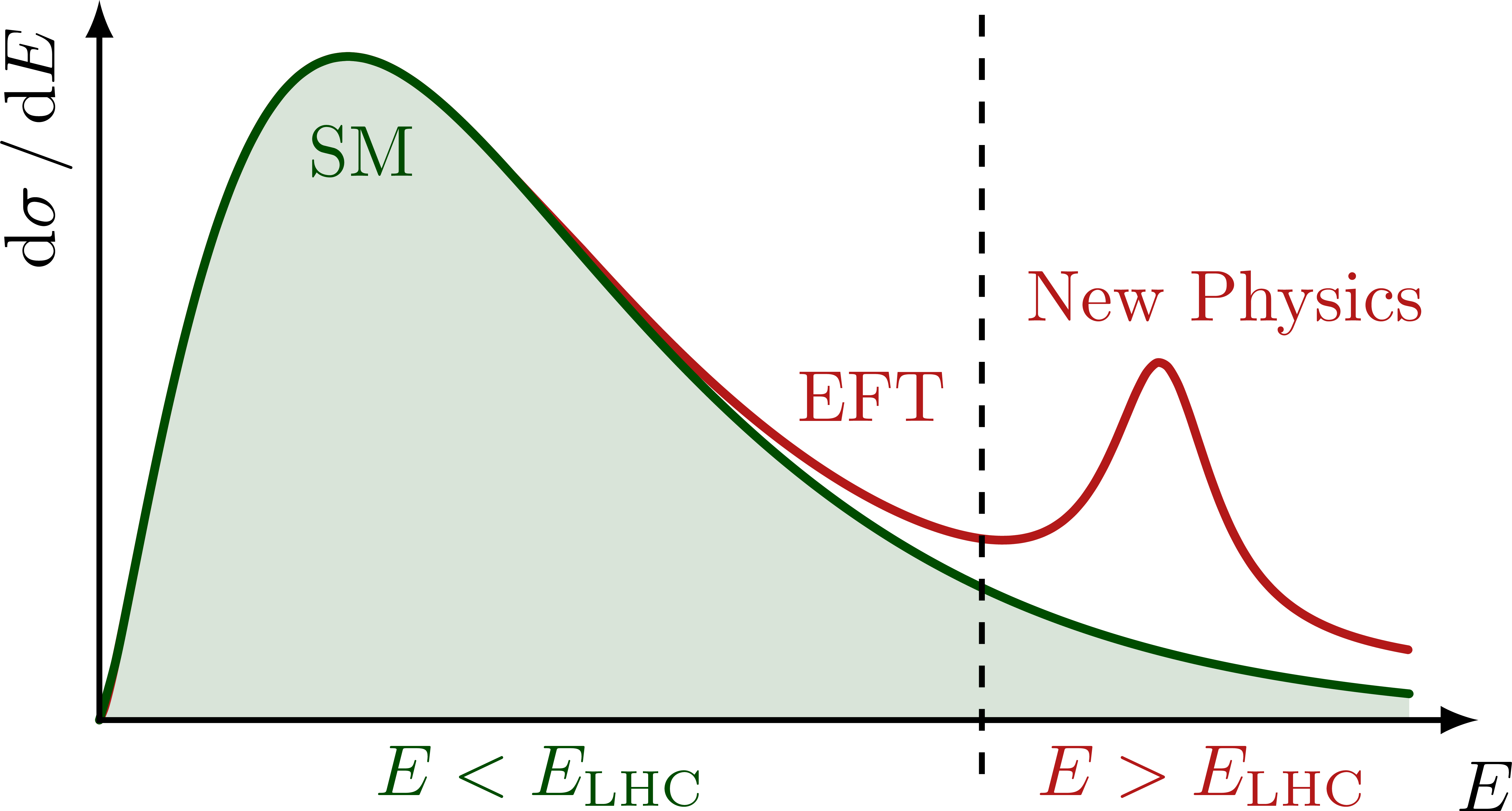
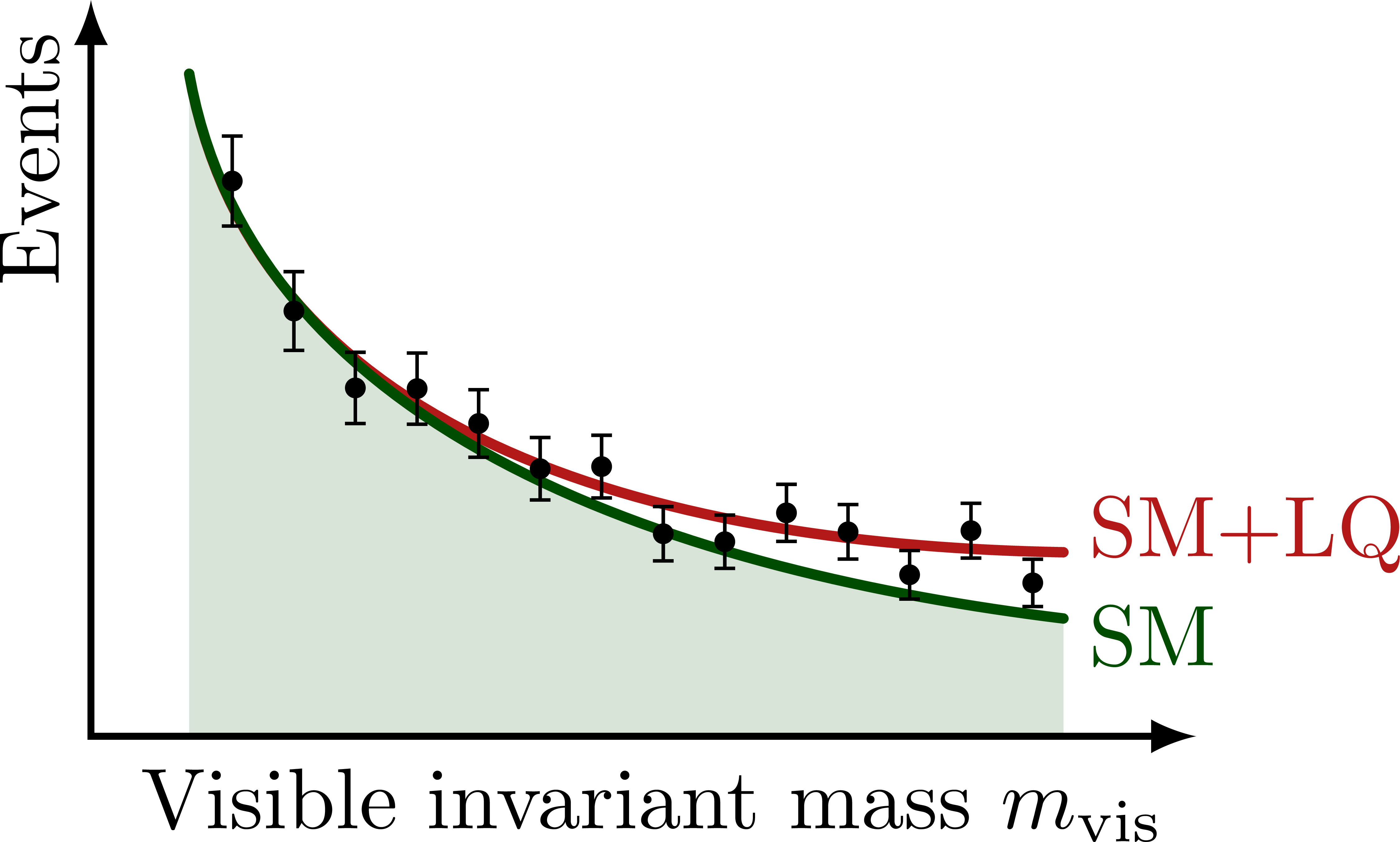
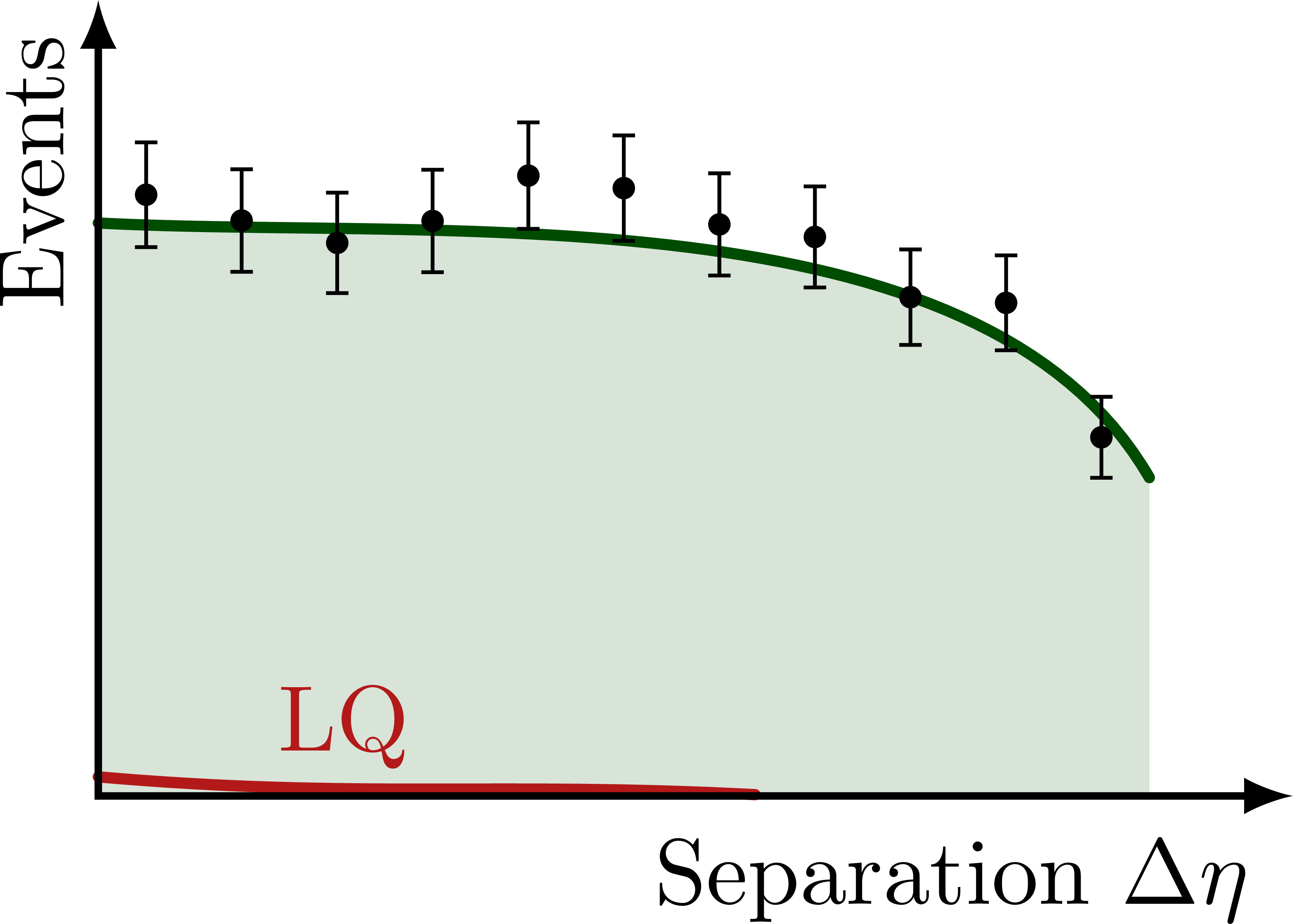
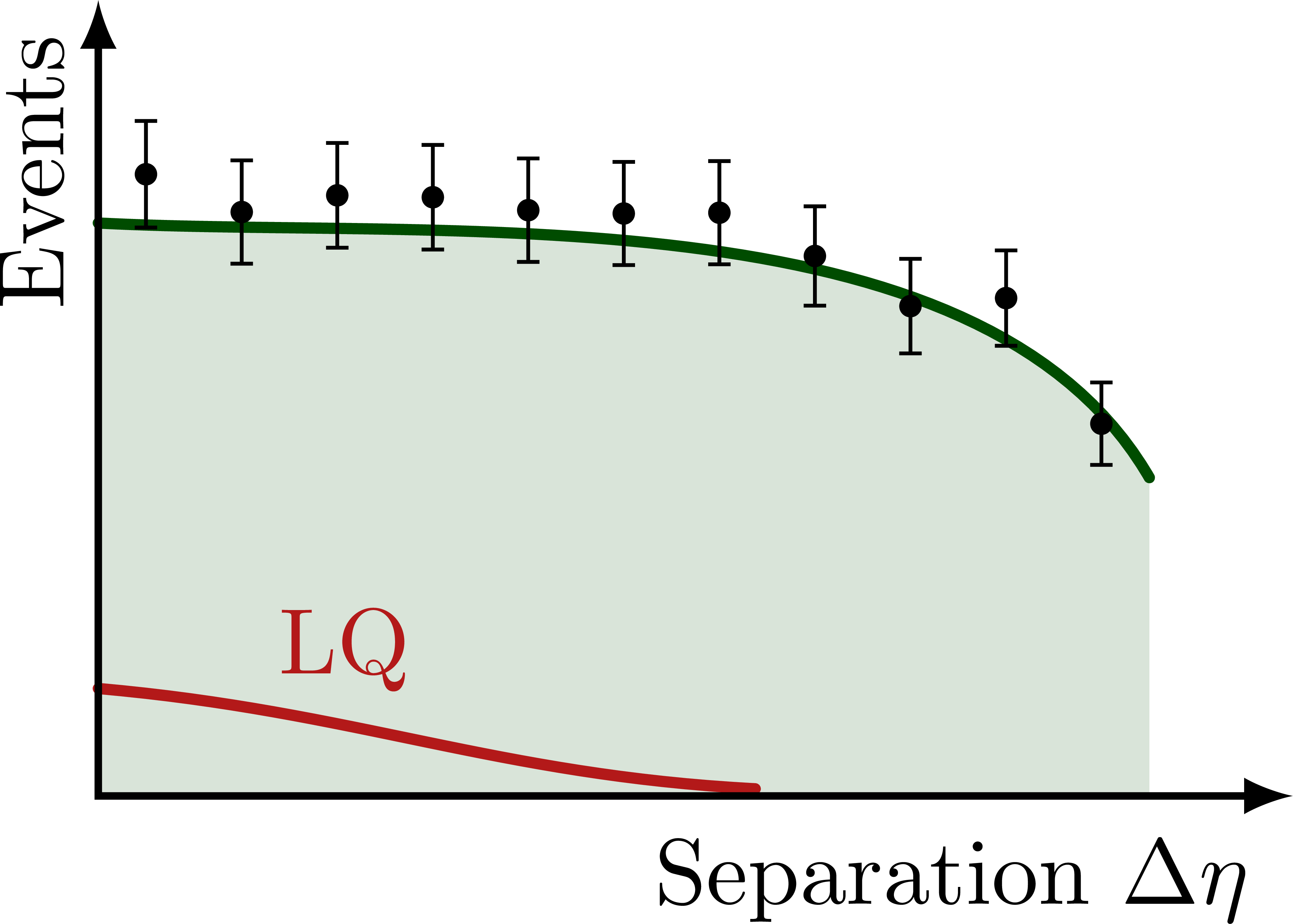
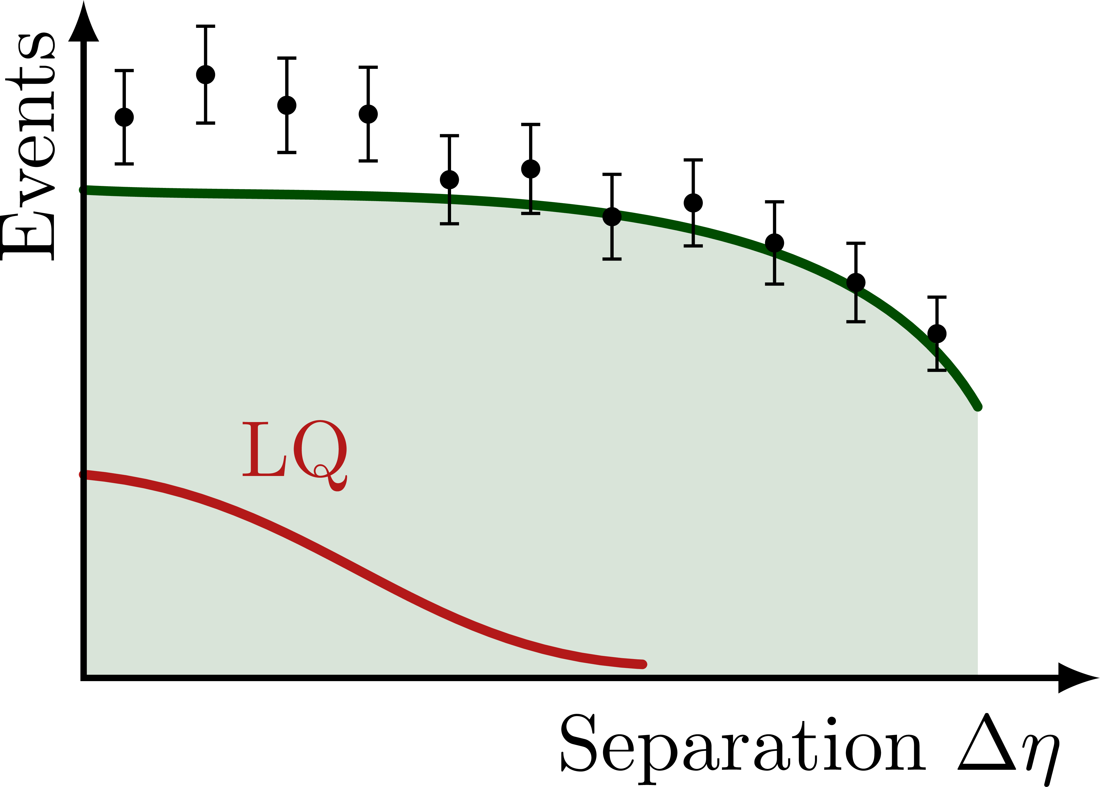
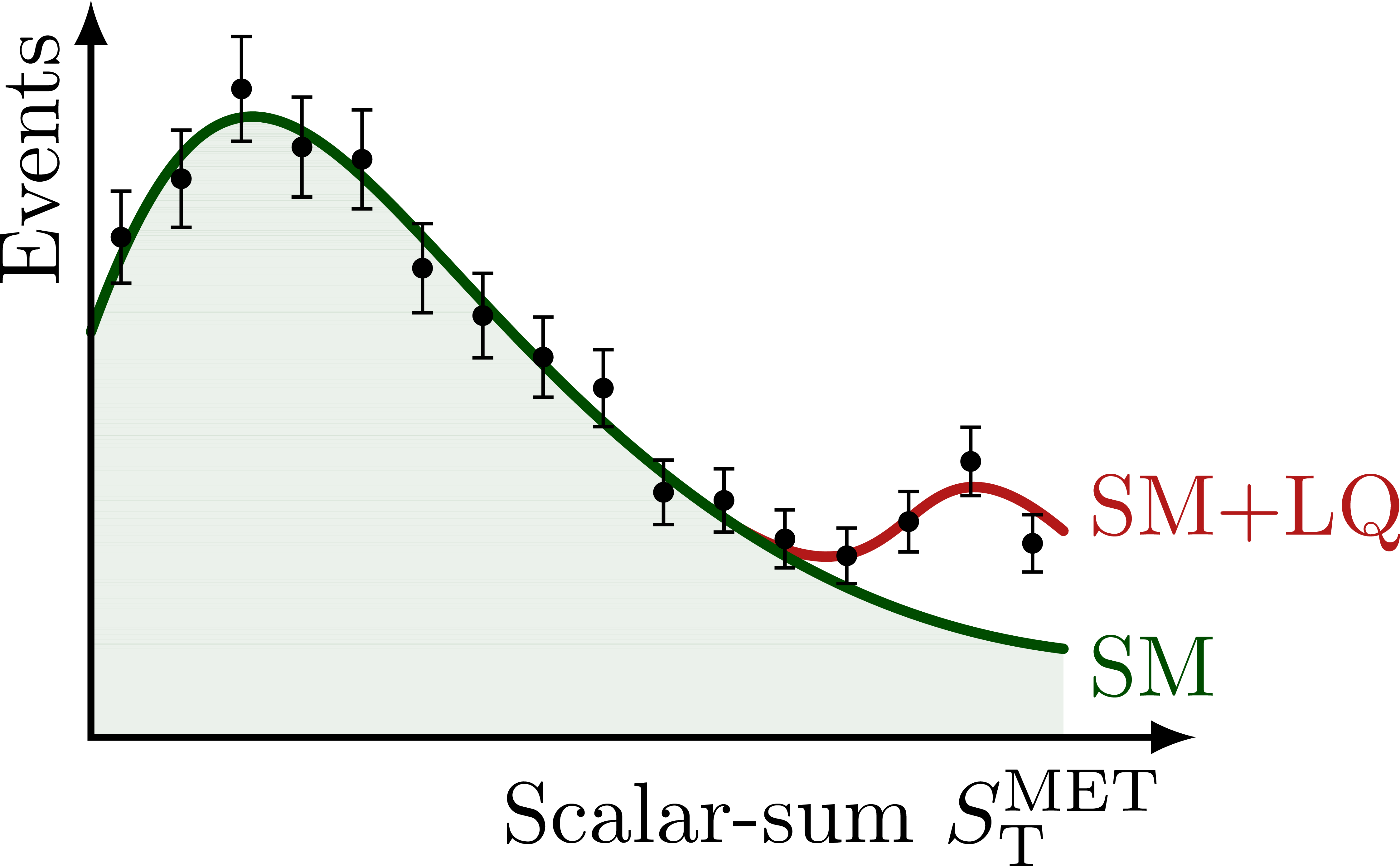
Illustration of the effects of new physics on the high-mass or high-pT tails in proton-proton collisions at detectors like CMS. Also shown are expected excesses in observed data, constructive vs. destructive interference, etc.

Edit and compile if you like:
% Author: Izaak Neutelings (September 2022)
\documentclass[border=3pt,tikz]{standalone}
\usepackage{amsmath}
\usepackage{physics} % for \dd
\usepackage{xfp} % higher precision (16 digits?) with fpeval
\usetikzlibrary{calc}
\usetikzlibrary{intersections}
\DeclareMathOperator{\Log}{Log}

% TIKZ
\tikzset{>=latex} % for LaTeX arrow head
\tikzstyle{curve}=[very thick,line cap=round]
\tikzstyle{dashed curve}=[curve,thick,dashed]
\pgfdeclarelayer{back} % to draw on background
\pgfsetlayers{back,main} % set order

% COLORS
\definecolor{myblue}{rgb}{.0,.13,.98} % 0,32,250
\definecolor{myred}{rgb}{.7,.1,.1}
\colorlet{mydarkred}{myred!80!black}
\colorlet{mydarkgreen}{green!30!black}
\colorlet{mylightgreen}{green!30!black!15}

%% FUNCTIONS
%\tikzset{declare function={% Kruskal-Szekeres coordinates
%  kruskalu(\x,\c) = {\fpeval{sqrt(\x*\x+(\c/2-1)*exp(\c/2))}};%
%}}

% DRAW RANDOM DATA POINTS
\def\yerrscale{0.26} % scale fluctuations
\def\ybarscale{0.7} % scale error bars
\def\wbar{1.2pt} % width of line at end of error bar
\def\drawdata[#1](#2:#3:#4){ % add data around named path
  \def\Ndata{#2} % number of data points
  \pgfmathsetmacro\xmindata{#3} % xmin for graph
  \pgfmathsetmacro\xmaxdata{#4} % xmax for graph
  %\pgfmathsetmacro\wbar{0.2*\xmaxdata/\Ndata} % width of line at end of error bar
  \foreach \i [evaluate={
    \x=\xmindata+(\i-0.5)*(\xmaxdata-\xmindata)/\Ndata;
  }] in {1,...,\Ndata}{
    \message{^^J N=\Ndata, i=\i, x=\x}
    \path[name path=vline] (\x,0) -- (\x,\ymax);
    \path[name intersections={of=#1 and vline, name=i}]
      coordinate (Pdata) at ($(i-1)+(0,{0.3*(rand)/2})$);
    \fill (Pdata) circle(1.2pt);
    \draw let \p1 = (Pdata) in % calculate y coordinate
      (Pdata) --++ (0,{\ybarscale*sqrt{\y1}}) coordinate(Pup)
      (Pdata) --++ (0,{-\ybarscale*sqrt{\y1}}) coordinate(Pdn)
      (Pup)++(\wbar,0) --++ (-2*\wbar,0)
      (Pdn)++(\wbar,0) --++ (-2*\wbar,0);
  }
}

\begin{document}


% HIGH-PT TAILS
\foreach \x in {m_{\ell\ell},p_\mathrm{T}^{\ell\ell}}{
\begin{tikzpicture}[scale=1]
  \message{^^JHigh-pt tails}
  \def\xmax{4.5} % x axis maximum
  \def\ymax{3.0} % y axis maximum

  % AXES
  \draw[<->,thick]
    (\xmax,0) node[below left] {$\x$}
    -| (0,\ymax) node[above left,rotate=90] {$\dd{\sigma}/\dd{\x}$};

  % CURVES
  \draw[curve,myred]
    (0.1*\xmax,0.9*\ymax) to[out=-80,in=179,looseness=0.98] (0.88*\xmax,0.25*\ymax)
    node[above=2,right=-1] {NP};
  \draw[curve,mydarkgreen]
    (0.1*\xmax,0.9*\ymax) to[out=-80,in=173,looseness=0.93] (0.88*\xmax,0.16*\ymax)
    node[below=2,right=-1] {SM};

\end{tikzpicture}}


% HIGH-PT TAILS - LOG-LOG
\foreach \x in {m_{\ell\ell},p_\mathrm{T}^{\ell\ell}}{
\begin{tikzpicture}[scale=1]
  \message{^^JHigh-pt tails (log-log)}
  \def\xmax{4.0} % x axis maximum
  \def\ymax{3.0} % y axis maximum
  \coordinate (A) at (0.1*\xmax,0.9*\ymax);

  % AXES
  \draw[<->,thick]
    (\xmax,0) node[below left] {$\Log\left[ \x \right]$}
    -| (0,\ymax) node[above left,rotate=90] {$\Log\left[ \dd{\sigma}/\dd{\x}\right]$};

  %%%% INTERSECTION
  %%%\def\pathSM{(A) to[out=-10,in=130,looseness=0.75] (0.85*\xmax,0.15*\ymax)}
  %%%\path[name path=line1] (0,0) -- (\xmax,\ymax);
  %%%\path[name path=line2] \pathSM;
  %%%\path[name intersections={of=line1 and line2, name=i}]
  %%%  (i-1) --++ (30:0.04) coordinate(P)
  %%%  (i-1) --++ (-140:0.05) coordinate(P'); % small offset
  %%%\fill (P) circle(1pt);
  %%%\fill (P') circle(1pt);

  % CURVES
  \draw[curve,mydarkgreen]
    (A) to[out=-10,in=130,looseness=0.75]
    node[pos=0.55] (P) {} (0.85*\xmax,0.15*\ymax)
    node[below=2,right=-1] {SM};
  \begin{pgfonlayer}{back} % draw on back
    \draw[curve,myred]
      (A) to[out=-10,in=142,looseness=0.80]
      ($(P)+(30:0.04)$) to[out=-38,in=170,looseness=0.90] (0.87*\xmax,0.37*\ymax)
      %(P) to[out=-38,in=170,looseness=0.90] (0.87*\xmax,0.37*\ymax)
      node[below=2,right=-1] {NP};
    \draw[dashed curve,mydarkred]
      (A) to[out=-10,in=140,looseness=0.9]
      ($(P)+(-140:0.05)$) to[out=-40,in=175,looseness=1.1] (0.87*\xmax,0.32*\ymax);
      %(P') to[out=-40,in=175,looseness=1.1] (0.87*\xmax,0.32*\ymax);
  \end{pgfonlayer}

  % LEGEND
  \draw[curve,myred,thick]
    (0.58*\xmax,0.92*\ymax) --++ (0.06*\xmax,0)
    node[right,scale=0.7] {Constructive};
  \draw[dashed curve,dotted,mydarkred]
    (0.58*\xmax,0.82*\ymax) --++ (0.06*\xmax,0)
    node[right,scale=0.7] {Destructive};

\end{tikzpicture}}


% HIGH-MASS TAILS with resonance
\foreach \fillSM in {0,1}{
\begin{tikzpicture}[scale=1]
  \message{^^JHigh-pt tails with resonance}
  \def\xmax{6.7} % x axis maximum
  \def\ymax{3.5} % y axis maximum

  %%%% CURVES
  %%%\draw[curve,myred]
  %%%  (0.38*\xmax,0.65*\ymax) coordinate(A) % point of deviation
  %%%    to[out=-55,in=-110,looseness=0.8] (0.76*\xmax,0.42*\ymax) %circle(0.5pt)
  %%%    to[out=70,in=180,looseness=0.45] (0.79*\xmax,0.58*\ymax) %circle(0.5pt)
  %%%    to[out=0,in=100,looseness=0.45] (0.815*\xmax,0.43*\ymax) %circle(0.5pt)
  %%%    to[out=-80,in=170,looseness=0.9] (0.96*\xmax,0.15*\ymax);
  %%%\draw[curve,mydarkgreen]
  %%%  (0,0) to[out=70,in=180,looseness=0.7] (0.23*\xmax,0.9*\ymax) %circle(1pt)
  %%%    node[below=4] {SM}
  %%%    to[out=0,in=125,looseness=1] (A) %circle(1pt)
  %%%    to[out=-55,in=170,looseness=1] (0.96*\xmax,0.1*\ymax);

  % CURVES (using functions)
  \pgfmathsetmacro\GamBW{0.14^2/4} % Gamma^2/4
  \def\SMcurve{\fpeval{1.6e2*\x^1.4*exp(-\x^0.93/1.35e-1)}}
  \def\BWpeak{\fpeval{1.3*\GamBW/((\x^2-0.77^2)^2+\GamBW)}} % Breit-Wigner
  \ifnum\fillSM=1
    \fill[mylightgreen,smooth,samples=80,domain=0:0.95]
      plot (\x*\xmax,{\SMcurve}) |- (0,0);
  \fi
  \draw[curve,myred,smooth,samples=80]
    plot[domain=0:0.3] (\x*\xmax,{\SMcurve}) --
    plot[domain=0.35:0.95] (\x*\xmax,{\SMcurve+0.25*max(0,\x-0.35)+\BWpeak});
  \draw[curve,mydarkgreen,smooth,samples=80,domain=0:0.95]
    plot (\x*\xmax,{\SMcurve});

  % AXES
  \draw[<->,thick]
    (\xmax,0) node[right=1,below=2] {$E$} %m_{\ell\ell}
    -| (0,\ymax) node[above left,rotate=90] {$\dd{\sigma}/\dd{E}$}; %m_{\ell\ell}

  % REGIONS
  \draw[thick,dashed]
    (0.64*\xmax,-0.075*\ymax) --++ (0,1.06*\ymax);
  \node[mydarkgreen,below] at (0.19*\xmax,0.86*\ymax) {SM};
  \node[myred,left=4,align=center]
    at (\xmax,0.58*\ymax) {New Physics};
  \node[myred,above,rotate=0] at (0.56*\xmax,0.38*\ymax) {EFT};
  \node[mydarkgreen,below,rotate=0] at (0.32*\xmax,0) {$E<E_\text{LHC}$};
  \node[myred,below,rotate=0] at (0.8*\xmax,0) {$E>E_\text{LHC}$};

\end{tikzpicture}}


% NONRES. LQ: INVARIANT MASS
\begin{tikzpicture}[scale=1]
  \message{^^Jmvis}
  \def\xmin{0.4} % x axis maximum
  \def\xmax{4.5} % x axis maximum
  \def\ymax{3.0} % y axis maximum
  \def\ybarscale{0.65} % scale error bars

  % CURVES
  \def\pathSM{
    (\xmin,0.9*\ymax) to[out=-80,in=173,looseness=0.93] (0.88*\xmax,0.16*\ymax)
  }
  \fill[mylightgreen]
    (\xmin,0) -- \pathSM |- cycle;
  \draw[curve,myred,name path=BSM]
    (\xmin,0.9*\ymax) to[out=-80,in=179,looseness=0.98] (0.88*\xmax,0.25*\ymax)
    node[above=2,right=-1] {SM+LQ};
  \draw[curve,mydarkgreen,name path=SM]
    \pathSM
    node[below=2,right=-1] {SM};

  % AXES
  \draw[<->,thick]
    (\xmax,0) node[below left] {Visible invariant mass $m_\text{vis}$} %m_{\tau\tau}^\text{vis}
    -| (0,\ymax)
    node[above left,rotate=90] {Events}; %$\dd{\sigma}/\dd{(m_\text{vis})}$};

  % DATA POINTS
  %\drawdata[SM](14:0:0.6*\xmax)
  \drawdata[BSM](14:0.1*\xmax:0.88*\xmax)

\end{tikzpicture}


% NONRES. LQ: SEPARATION DELTA ETA
\foreach \yf in {0.08,0.45,1}{
\begin{tikzpicture}[scale=1]
  \message{^^JDelta eta yf=\yf}
  \def\xmax{4.5} % x axis maximum
  \def\ymax{3.0} % y axis maximum

  % CURVES
  \def\pathSM{
    (0,0.72*\ymax) to[out=-3,in=120,looseness=0.8]
    %node[pos=0.8,above right=-1pt] {SM}
    (0.88*\xmax,0.4*\ymax)
  }
  \path[name path=BSM]
    (0,{(0.72+\yf*0.16)*\ymax}) to[out=-3,in=172,looseness=0.8]
    (0.46*\xmax,0.72*\ymax) to[out=-8,in=120,looseness=0.9]
    (0.88*\xmax,0.4*\ymax);
  \fill[mylightgreen]
    (0,0) -- \pathSM |- cycle;
  \draw[curve,mydarkgreen,name path=SM]
    \pathSM;
  %\begin{pgfonlayer}{back} % draw on back
  \draw[curve,myred]
    (0,\yf*0.30*\ymax) to[out=-5,in=177,looseness=1.0]
    node[pos=0.23,above right=-2pt] {LQ}
    (0.55*\xmax,\yf*0.02*\ymax);
  %\end{pgfonlayer}

  % DATA POINTS
  \drawdata[BSM](11:0:0.88*\xmax)
  %\drawdata[BSM](5:0.6*\xmax:0.88*\xmax)

  % AXES
  \draw[<->,thick]
    (\xmax,0) node[below left=1pt] {Separation $\Delta\eta$}
    -| (0,\ymax)
    node[above left,rotate=90] {Events}; %$\dd{\sigma}/\dd{(\Delta\eta)}$};

\end{tikzpicture}}


% STMET
\begin{tikzpicture}[scale=1]
  \message{^^JSTMET}
  \def\xmax{4.5} % x axis maximum
  \def\ymax{3.0} % y axis maximum
  \clip (-0.13*\xmax,-0.2*\ymax) rectangle (1.2*\xmax,1.05*\ymax);

  % CURVES
  \def\pathSM{
    (0,0.55*\ymax) to[out=70,in=173,looseness=1.6]
    coordinate[pos=0.8] (M)
    (0.88*\xmax,0.12*\ymax)
  }
  \fill[mylightgreen]
    (0,0) -- \pathSM |- cycle;
  \draw[curve,mydarkgreen,name path=SM]
    \pathSM
    node[below=2,right=-1] {SM};
  \begin{pgfonlayer}{back} % draw on back
    \draw[curve,myred,name path=BSM]
      (M) to[out=-30,in=140,looseness=1.7]
      (0.88*\xmax,0.28*\ymax)
      node[above=2,right=-1] {SM+LQ};
  \end{pgfonlayer}

  % DATA POINTS
  \drawdata[SM](11:0:0.6*\xmax)
  \drawdata[BSM](5:0.6*\xmax:0.88*\xmax)

  % AXES
  \draw[<->,thick]
    (\xmax,0)
    node[below left] {Scalar-sum $S_\text{T}^\text{MET}$} %m_{\tau\tau}^\text{vis}
    -| (0,\ymax)
    node[above left,rotate=90] {Events}; %$\dd{\sigma}/\dd{(S_\text{T}^\text{MET})}$};

\end{tikzpicture}


% LEGEND
\begin{tikzpicture}[scale=1]
  \def\ybar{0.18}
  \def\wbar{1.6pt}
  \fill (0,0) circle(1.4pt);
  \draw[line width=0.7]
    (0,-\ybar) -- (0,\ybar)
    (-\wbar,\ybar) --++ (2*\wbar,0)
    (-\wbar,-\ybar) --++ (2*\wbar,0);
  \node[right=2pt] (0,0) {Observed data};
\end{tikzpicture}


\end{document}
Click to download: BSM_tails.tex • BSM_tails.pdf
Open in Overleaf: BSM_tails.tex


