")


This post contains Minkowski diagrams of flat spacetime with light cones to illustrate the causal structure, as well as graphical interpretations of Lorentz transformations (“boosts”), and more. Some figures were inspired by Very special relativity – An illustrated guide by Sander Bais. For more related figures made with TikZ, please see Relativity category.
Like all diagrams on this website, they were made with the TikZ package in LaTeX, and the full source code to reproduce them can be found at the end of this post. This page not meant as a guide or full explanation. An animated explanation of Lorentz transformation is can be found in this excellent YouTube video by ScienceClic. An excellent explanation of the Twin paradox with spacetime diagrams can be found in this YouTube video by FloatingHeadPhysics, as well as in this one by MinutePhysics.
Table of content:
- World lines
- Causal structure of Minkowski spacetime
- Coordinate transformations
- Simultaneity
- Time dilation
- Length contraction
- Paradoxes
- Hyperbolae
- Analogy to Euclidean rotation
- Lorentz factor
- Full code
World lines
Empty spacetime diagram.
Several spacetime world lines with different velocities.

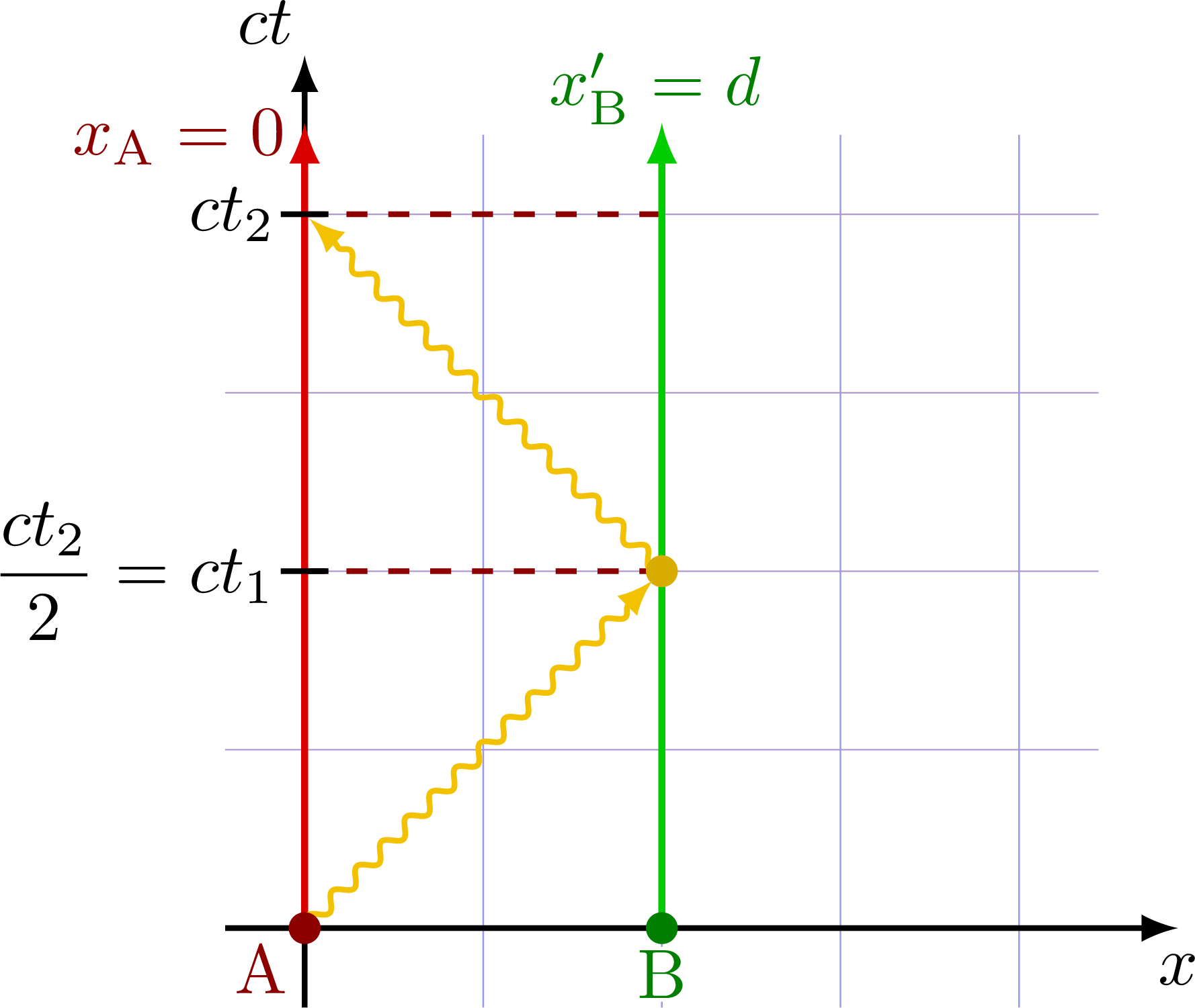
Two observers at rest (w.r.t. to each other) communicating by reflecting a light signal.
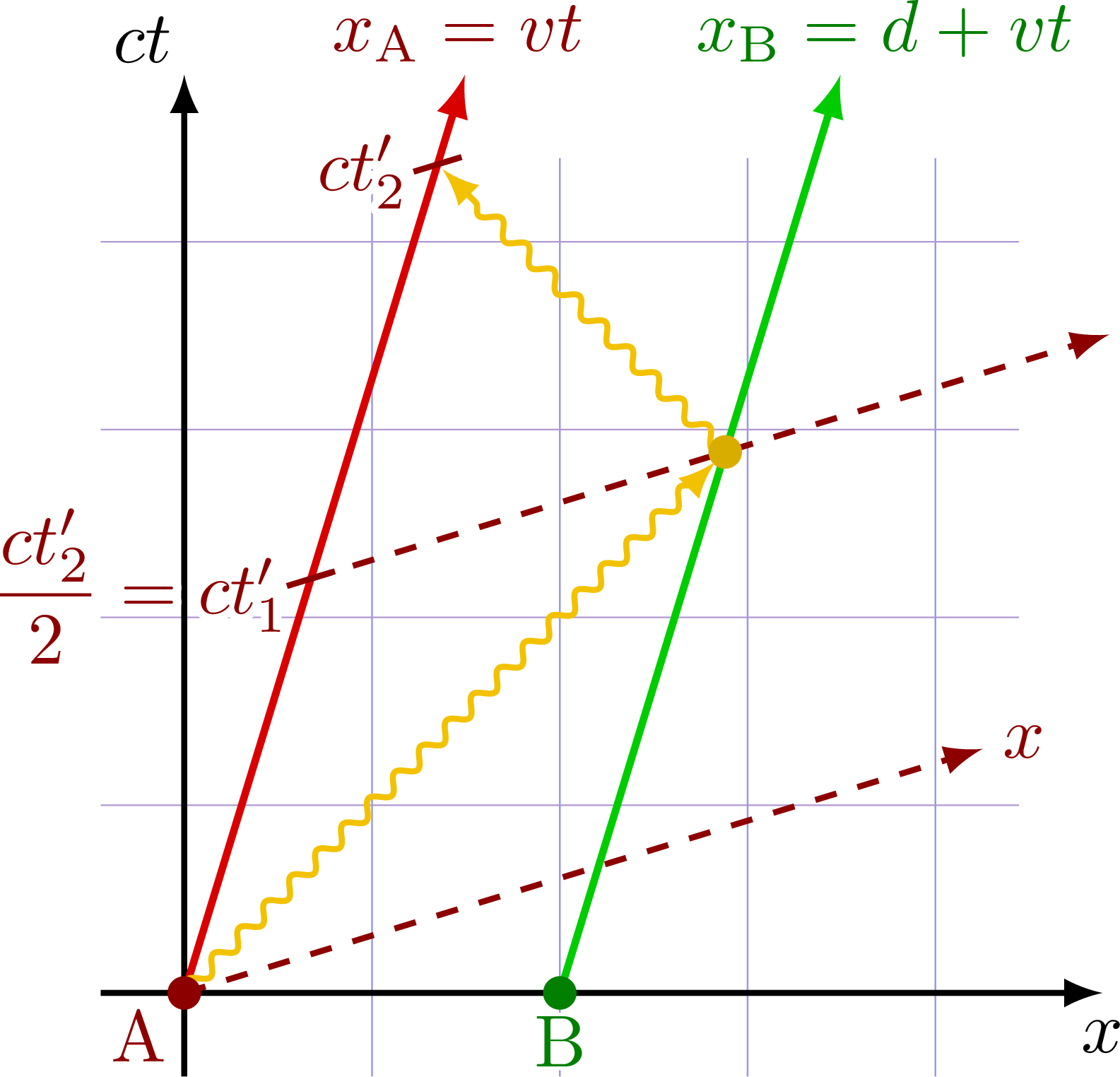
Derivation of the relativity of simultaneity with the thought experiment of two moving observers (with the red and green world lines) communicating with a light signal. Assuming the speed of light is c in all inertial frame of references (second postulate of special relativity), the dashed lines represent the plane of simultaneity. All events on a given dashed line happen at the same time from the point of view of the moving observers.
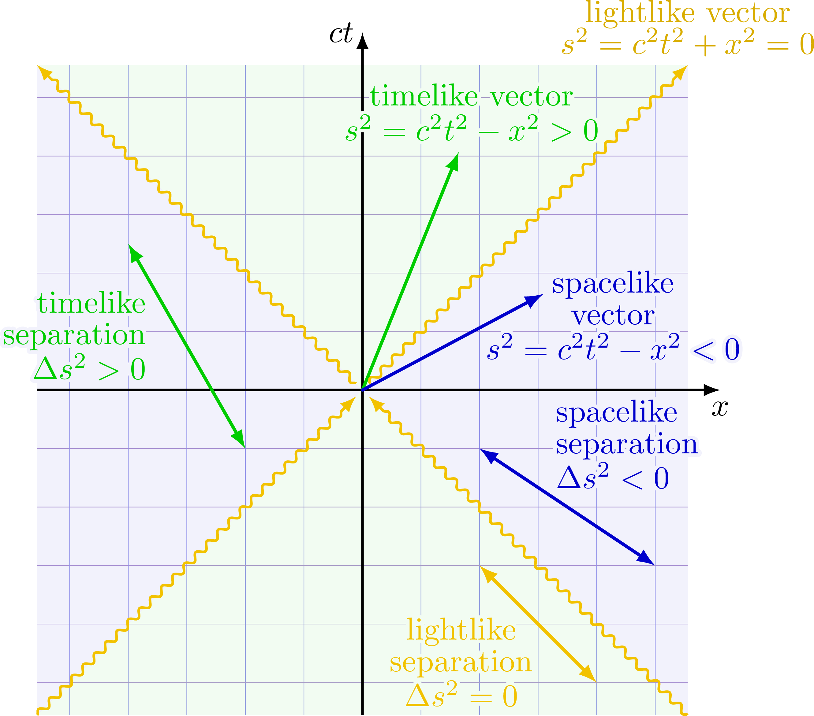
Causal structure of Minkowski spacetime
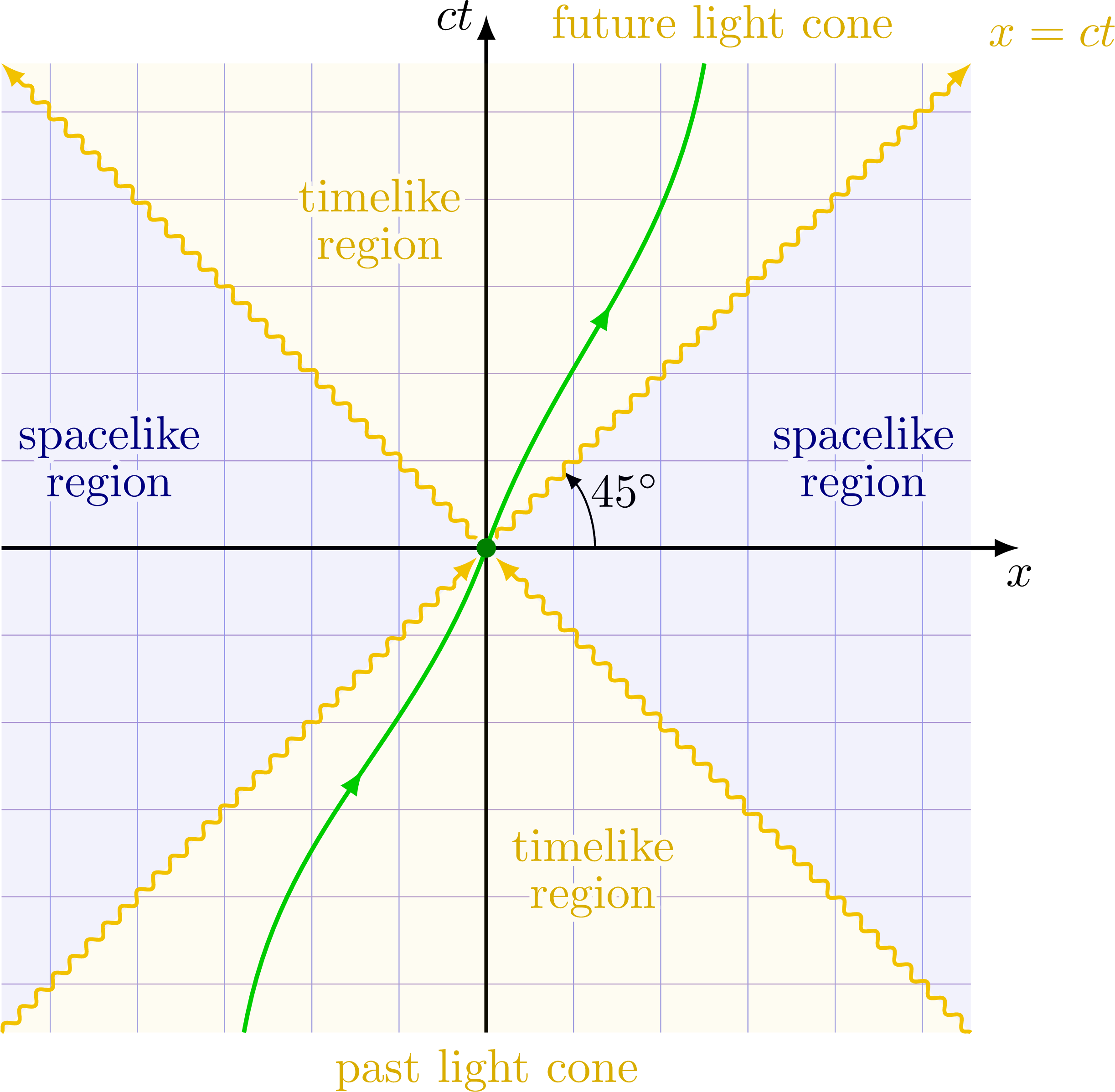
Future and past lightcone at a 45 degrees angle to illustrate the causal structure of Minkowski space.
Different types of spacetime vectors and separation: timelike (s2 > 0), spacelike (s2 = 0) and lightlike or null (s2 < 0).
Overlapping light cones of two observers separated in spacetime to illustrate the causal structure.

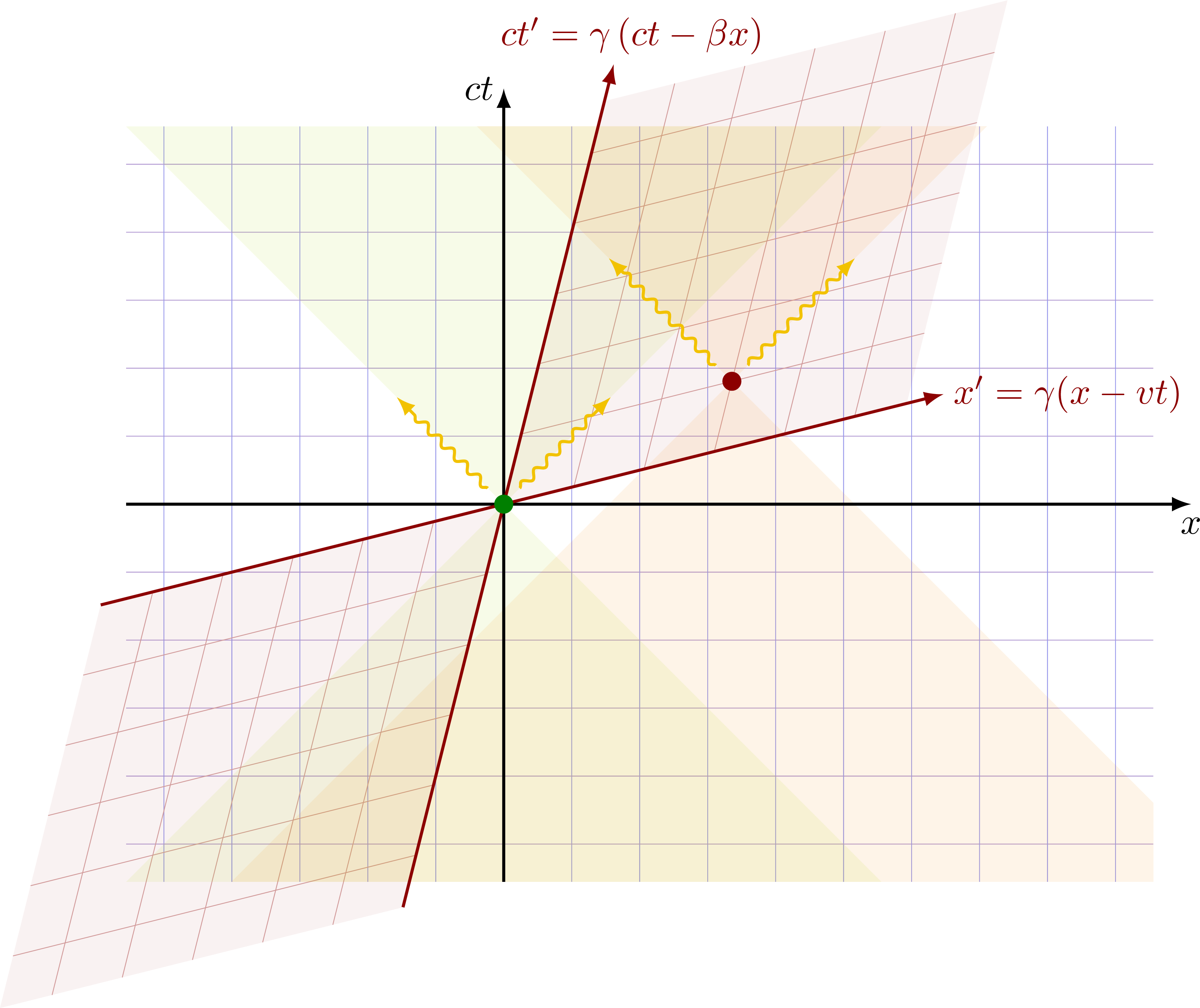
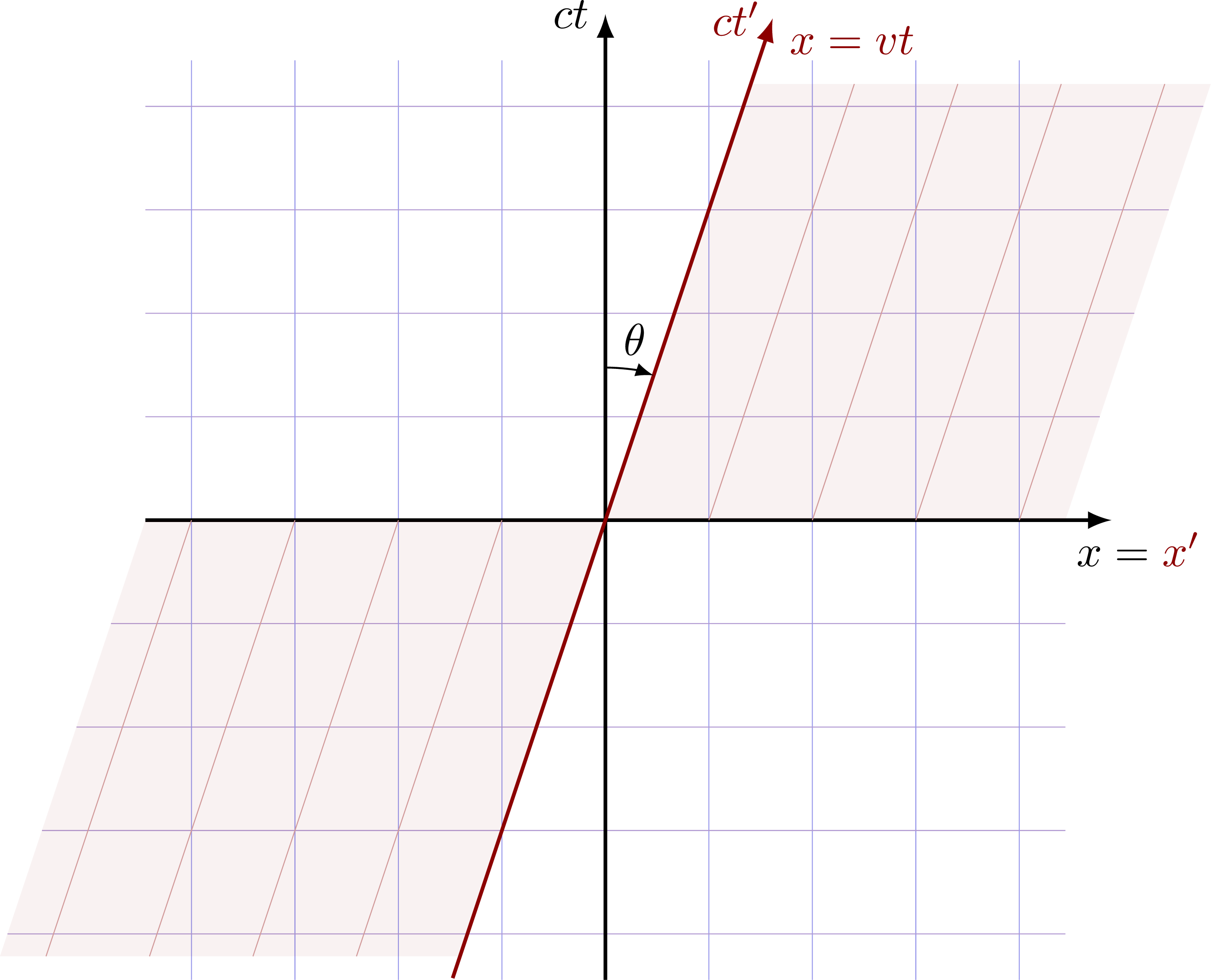
Coordinate transformations
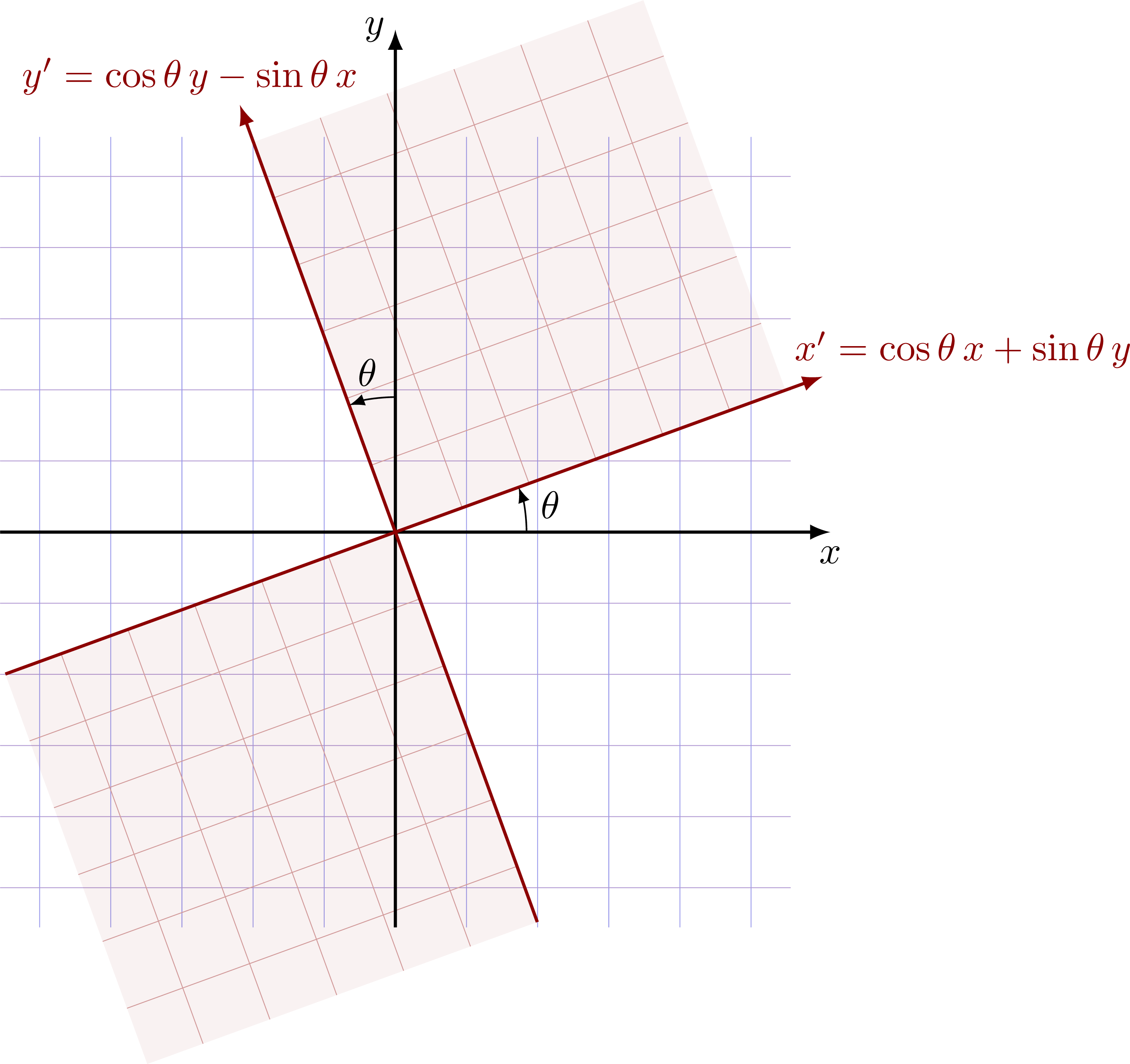
Simple 2D rotation in the (Euclidean) xy plane.
Galilean transformation for a moving frame. Clocks in both frames are equal (the grid lines at constant time ct and ct’ coincide).
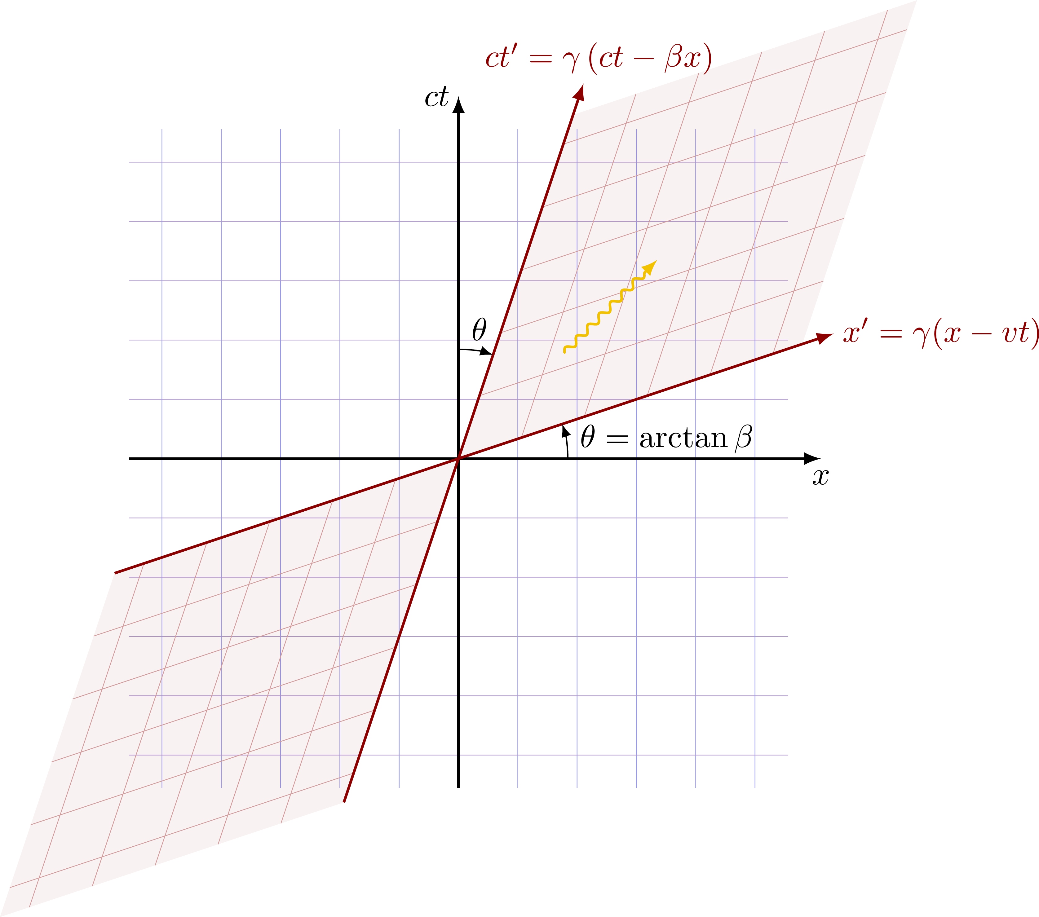
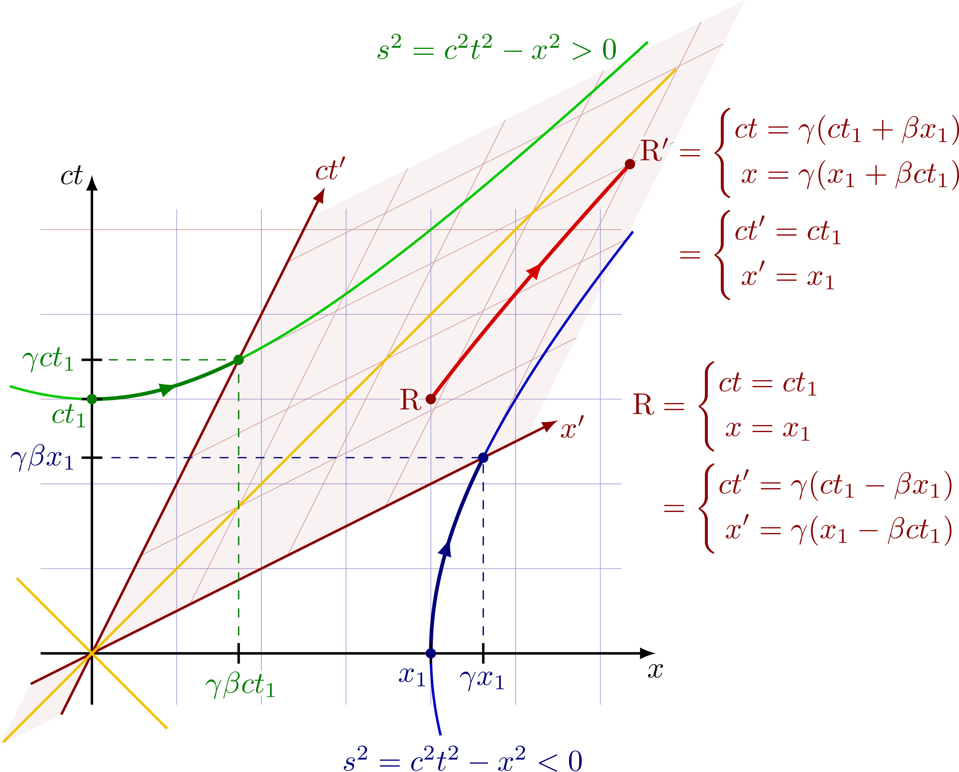
Lorentz transformation, or “boost”. Notice that the angle θ is given by the slope β = v/c = tanθ.
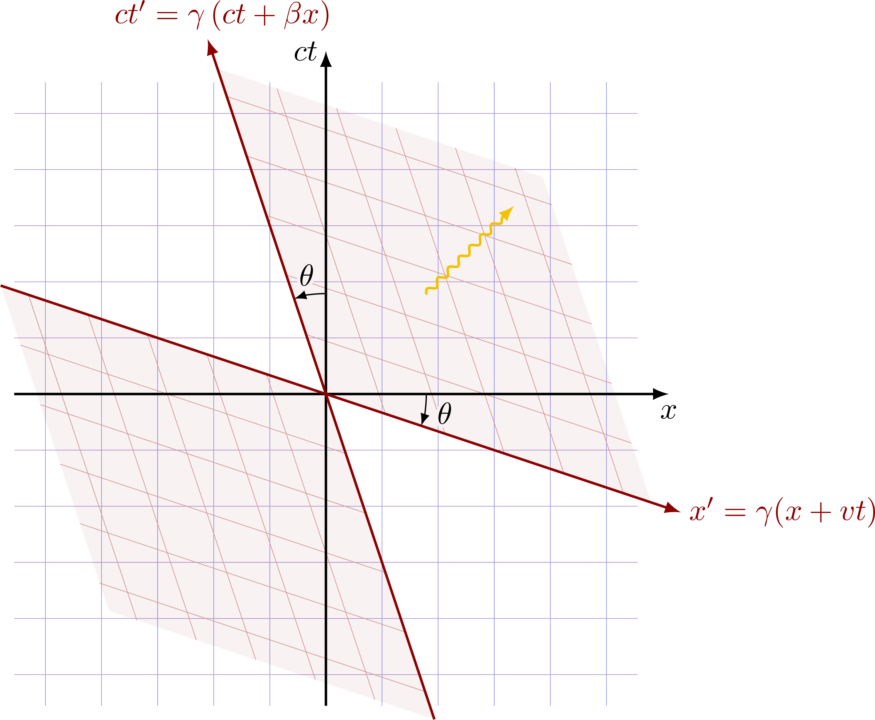
Inverse Lorentz transformation, or equivalently, if the boosted frame is moving to the left (in the negative x direction).
Simultaneity
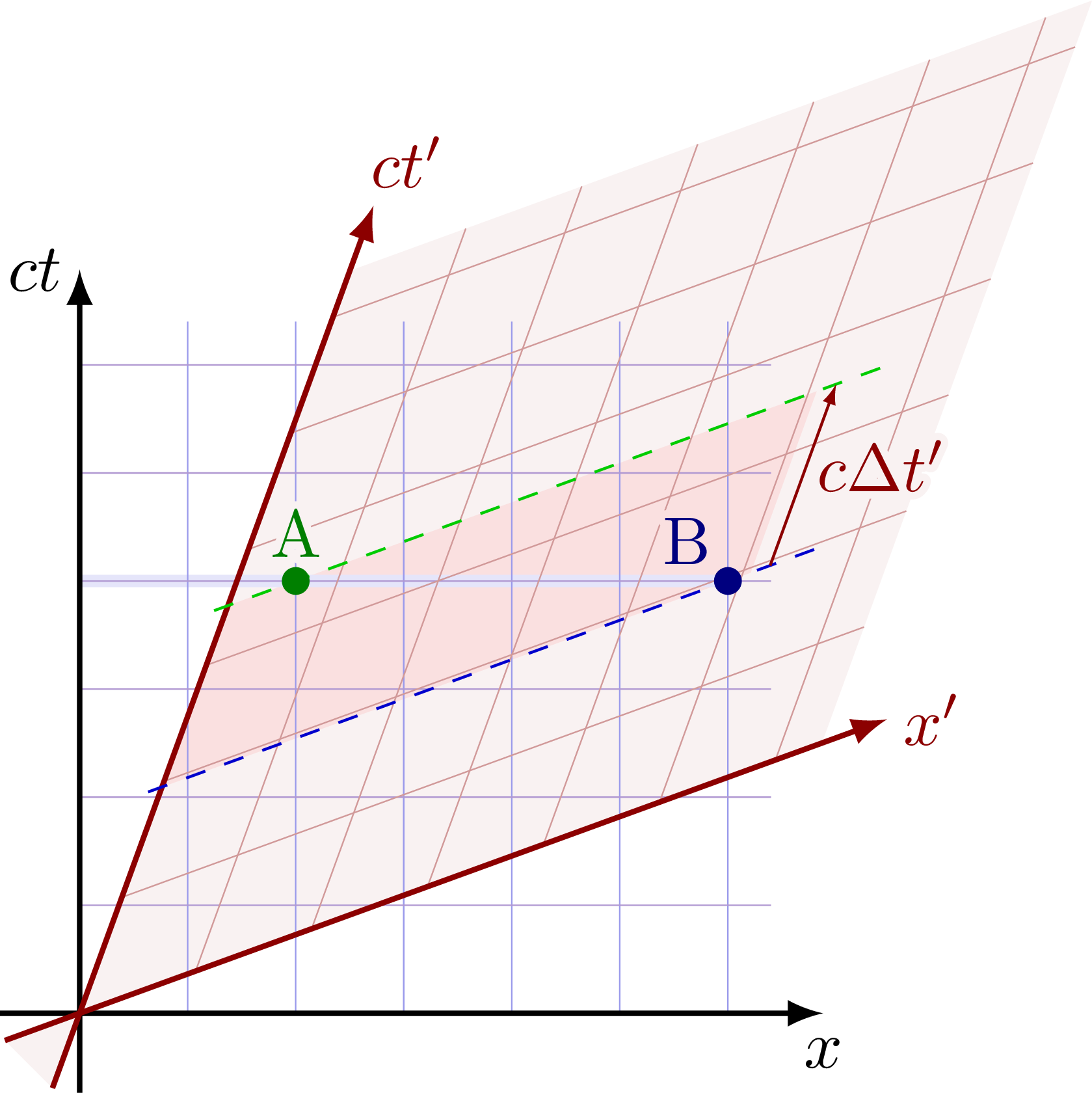
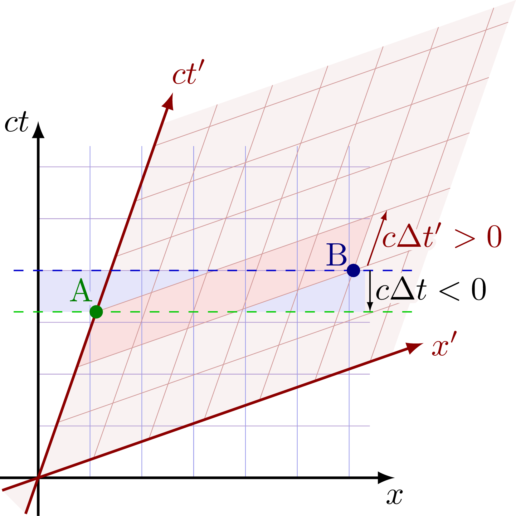
Events A and B are simultaneous in the rest frame S, but in the boosted frame S’, B happens before A.
Events A and B are simultaneous in the boosted frame S’, but in the rest frame S, A happens before B.
Relativity of simultaneity. Two observers experience events at in different order: In frame S, A happens before B, while in frame S’, B happens before A.
Time dilation
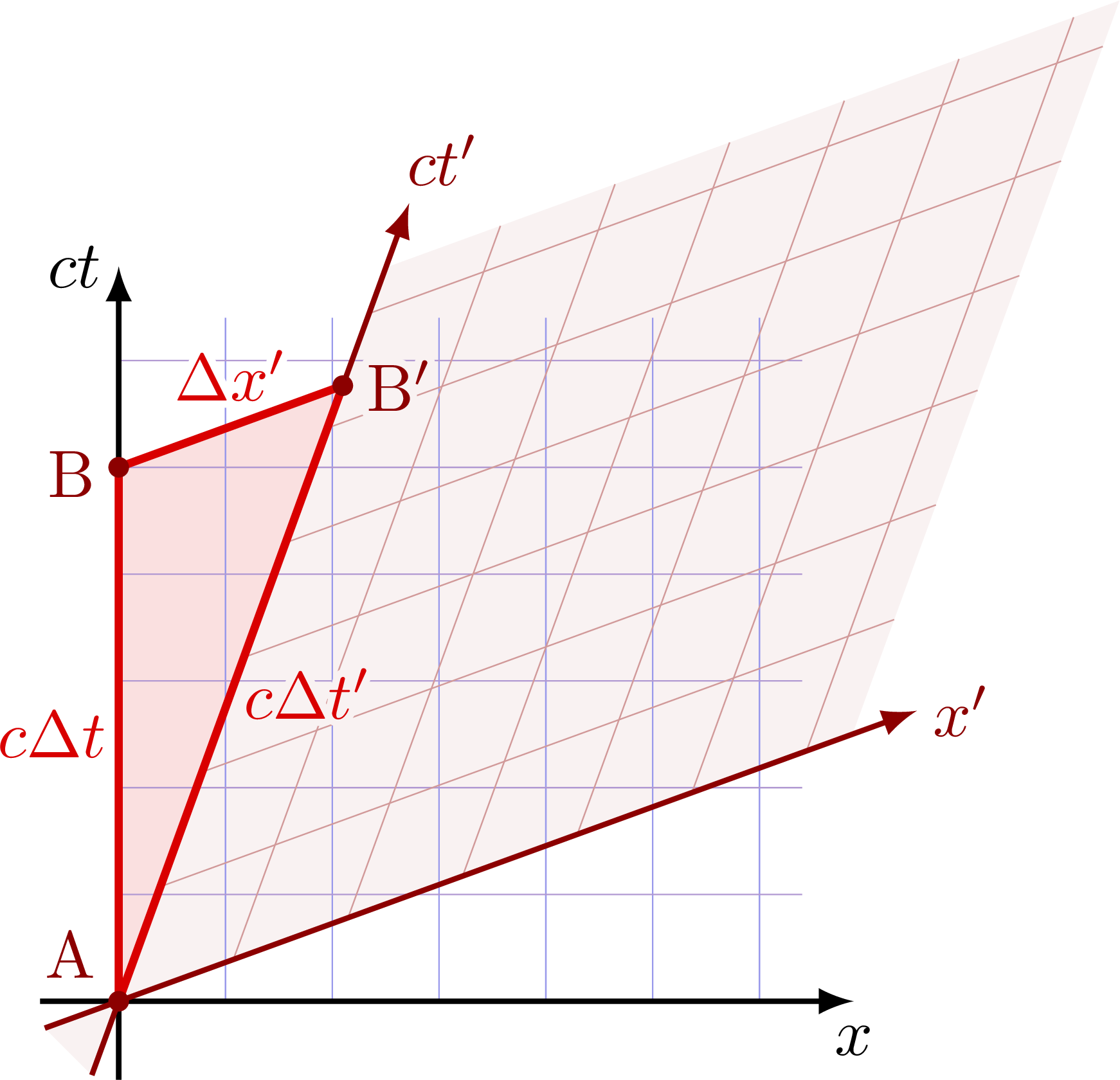
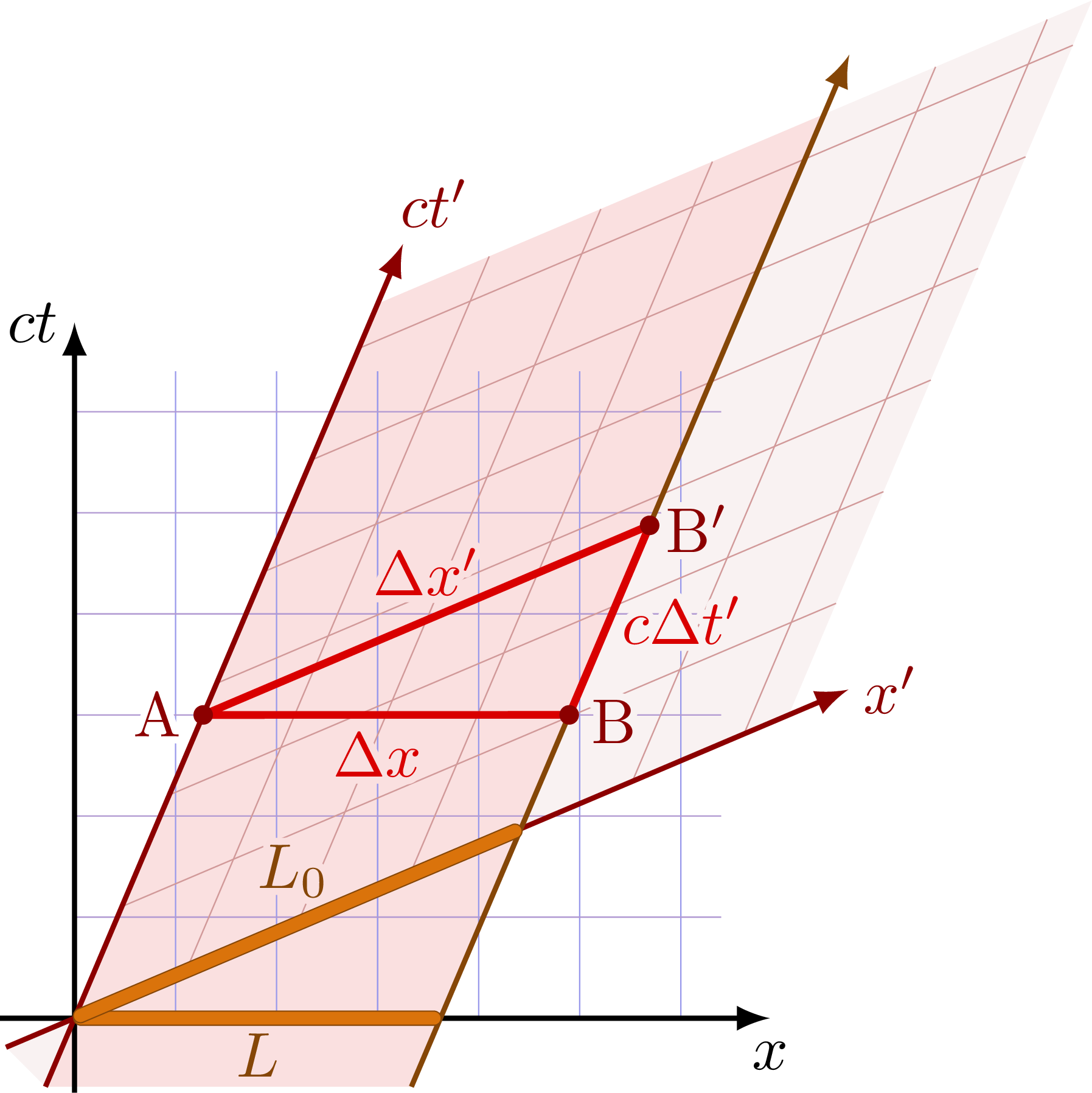
Time dilation in the boosted frame S’ for events at a fixed point of space in frame S. The time separation between A and B is longer in S’ than in S; Δt’ > Δt. The derivation is given in these lecture notes by Dr. Russell L. Herman.
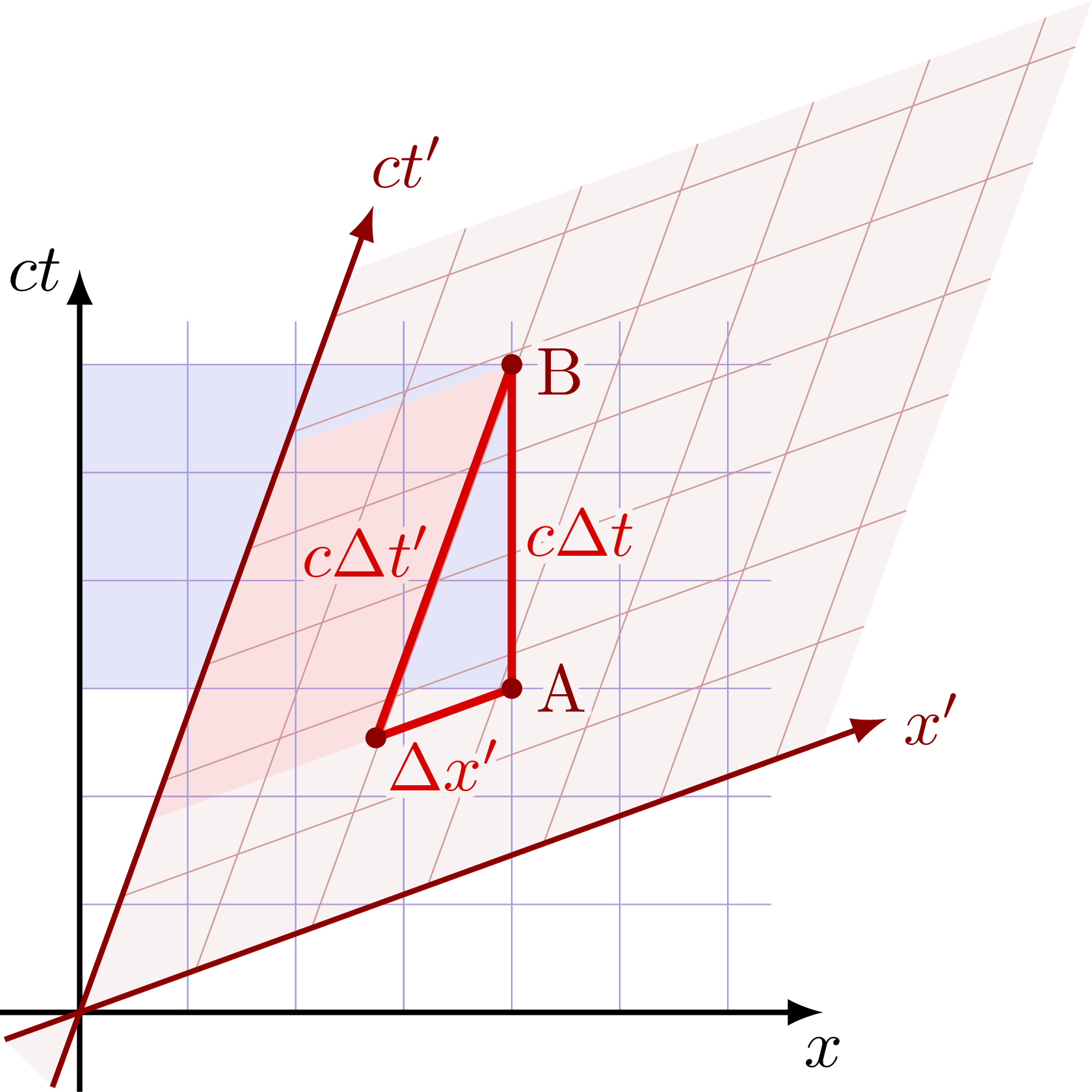
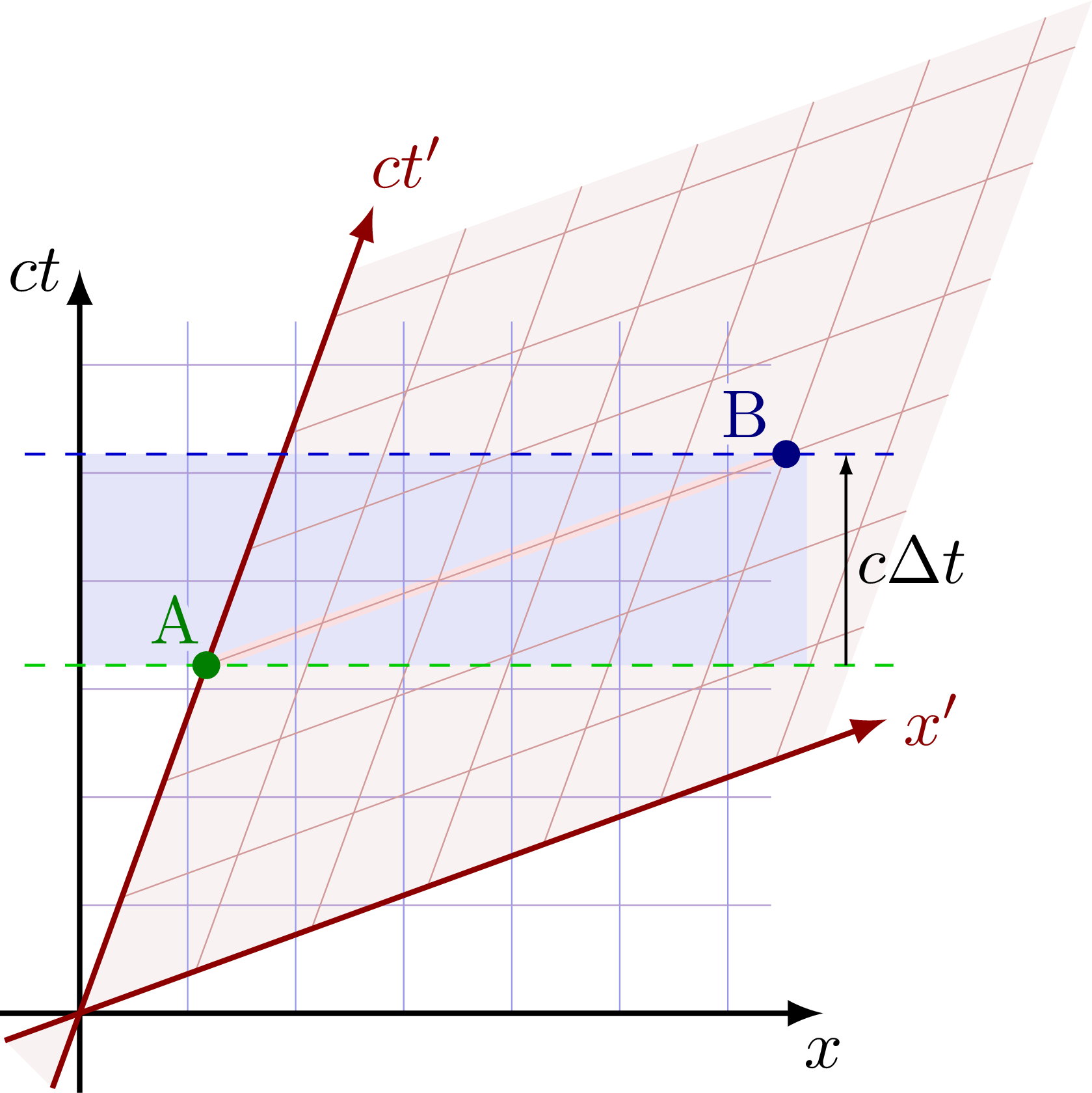
Time dilation for events at a fixed point of space in the boosted frame S’. The time separation between A and B is longer in S than in S’; Δt > Δt’.

Length contraction
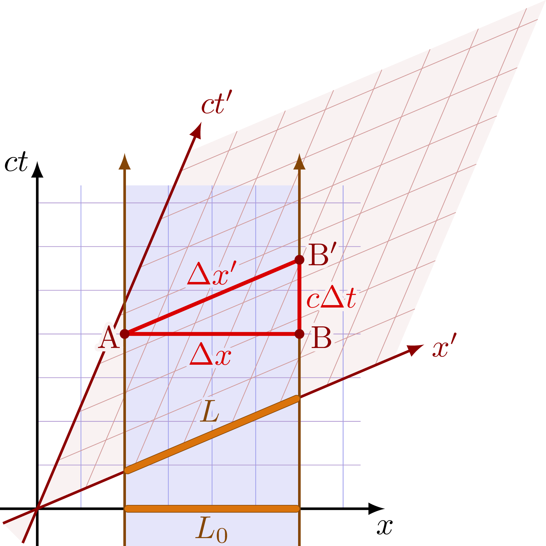
Length contraction of a rod at rest in frame S. The rod is shorter in the boosted frame S’, because it is moving relative to this frame. The derivation is given in these lecture notes.
Length contraction of a rod moving in frame S. The rod is shorter in the frame S’, because it is moving relative to this frame.
Paradoxes
Ladder paradox
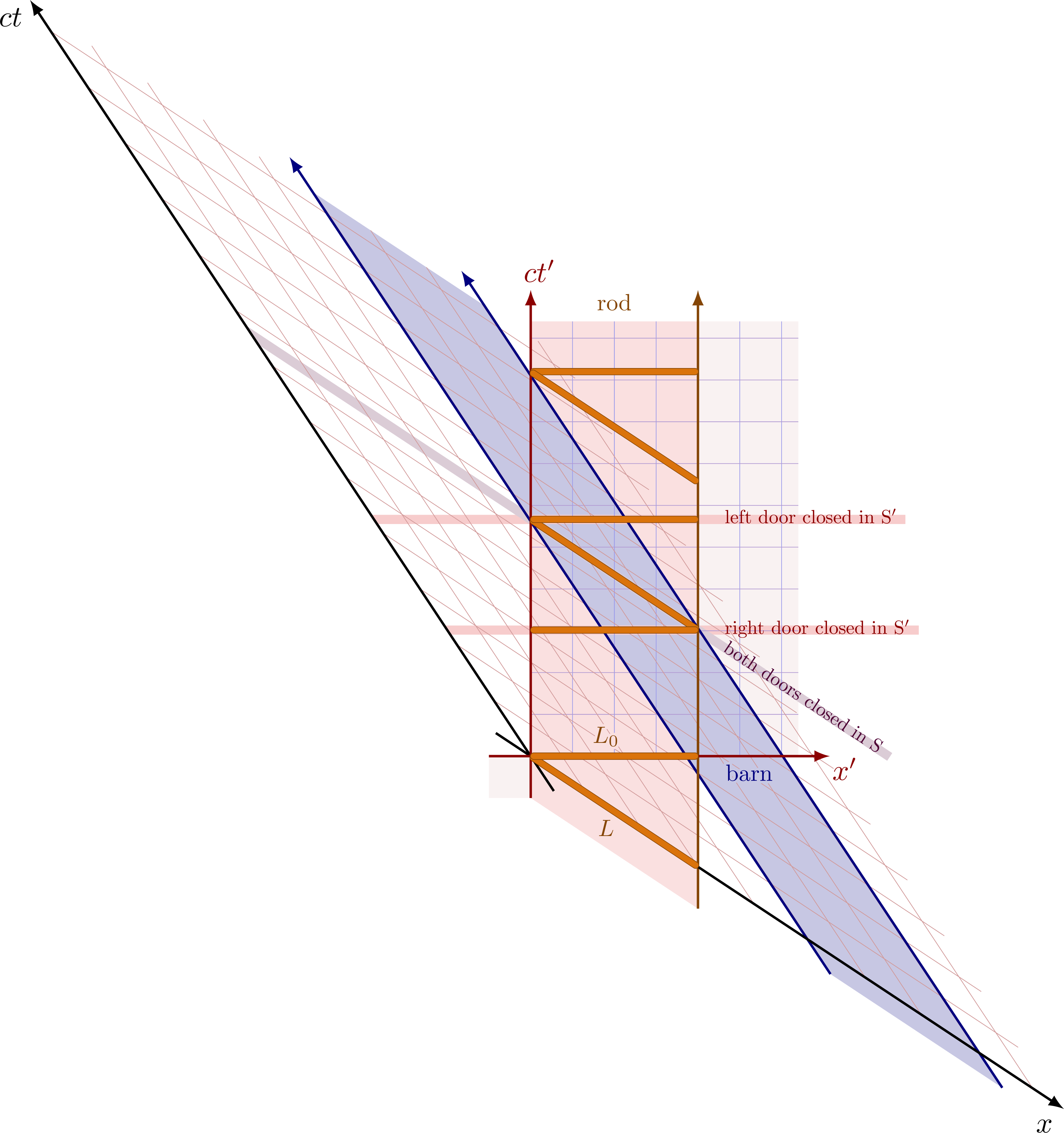
Ladder paradox: Due to length-contraction, a long ladder moving at relativistic speed is short enough to fit in a barn with both doors simultaneously closed. In the moving frame S’, however, the barn is contracted and cannot fit the ladder. The solution to the paradox is that the doors are never simultaneously closed in S’ due to the relativity of simultaneity.
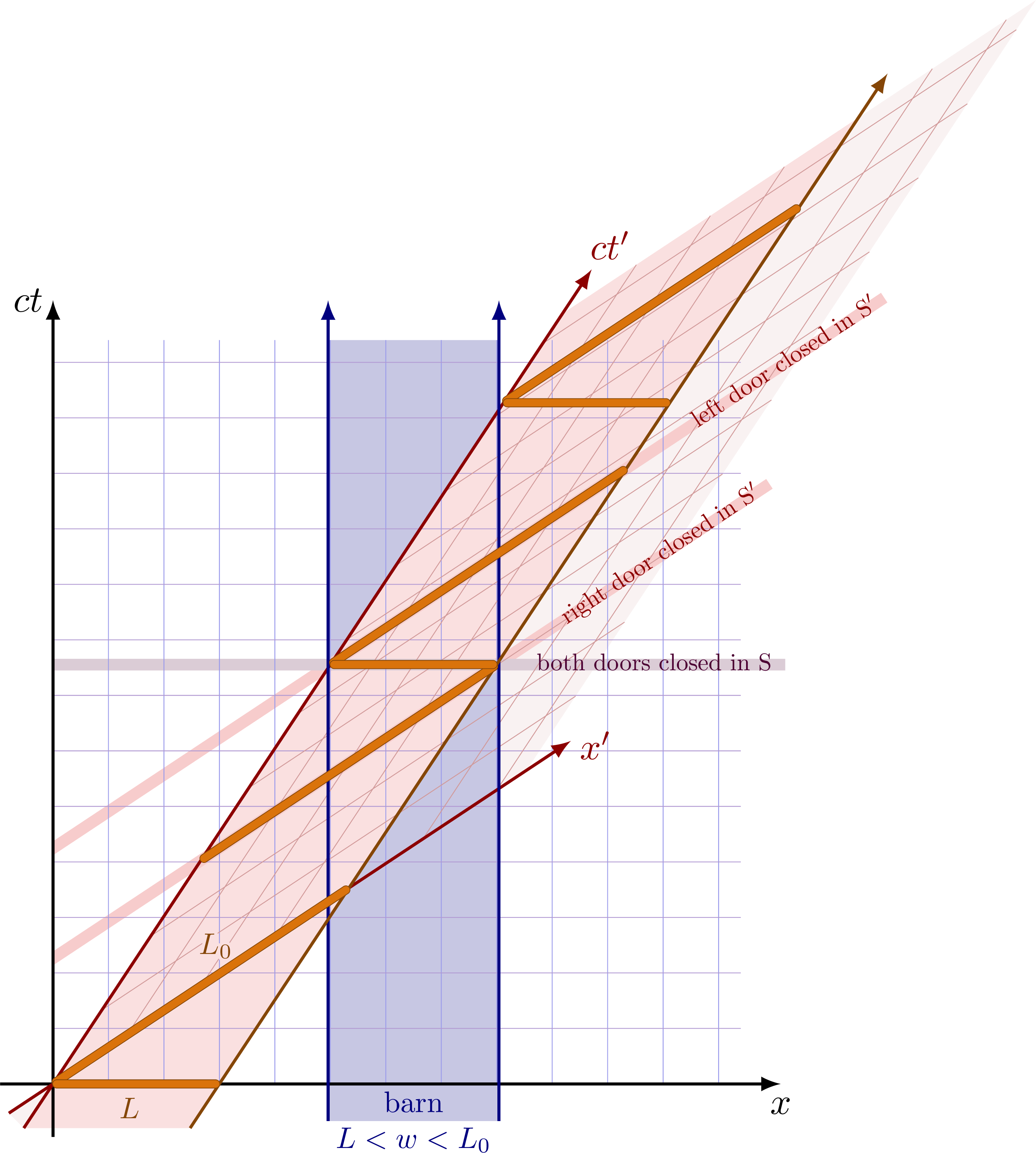
From the perspective of the observer in their rest frame S’, the barn is moving, and the doors are not closed simultaneously:
Twin paradox
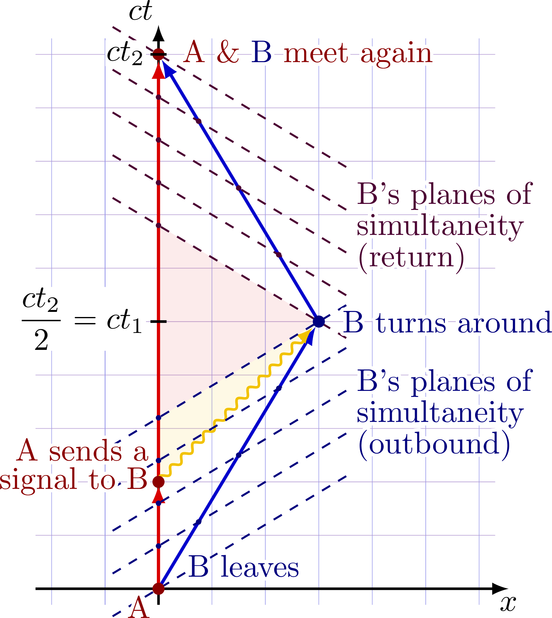
Below is an explanation of the Twin paradox using planes of simultaneity. An excellent explanation of the Twin paradox with spacetime diagrams can be found in this YouTube video by FloatingHeadPhysics, as well as in this one by MinutePhysics. It is also explained in full only the related Wikipedia page.
Twin Alice (A) stays stationary on Earth while twin Bob (B) makes a round trip with some large velocity v. From Alice’s perspective, Bob should be younger when he returns because of time dilation, Δt’ = Δt/γ < Δt. But if speed is relative, and Alice was traveling with a velocity v from Bob’s perspective, should Alice not be younger according to Bob? This is the paradox.
To resolve this apparent contradiction, one can analyze the spacetime diagrams, in particular by drawing Bob’s planes of simultaneity, i.e., the points that happen simultaneously in Bob’s frame (see the related section above).
The spacetime diagram shown below is Alice’s rest frame, where her worldine is shown as a red vector, while Bob’s world line is shown by two blue vectors moving at some fixed velocity v first away and then back towards Alice. In Alice’s reference frame, Bob’s planes of simultaneity are tilted (dashed lines). Because Bob changes frames, there will be a “gap” between the planes of simultaneity before and after he turns around. This means that Alice’s has a proper time Δt that is larger than Bob’s proper time Δt’ = Δt/γ < Δt, even in Bob’s own frame. This gap is shaded in the diagram below.
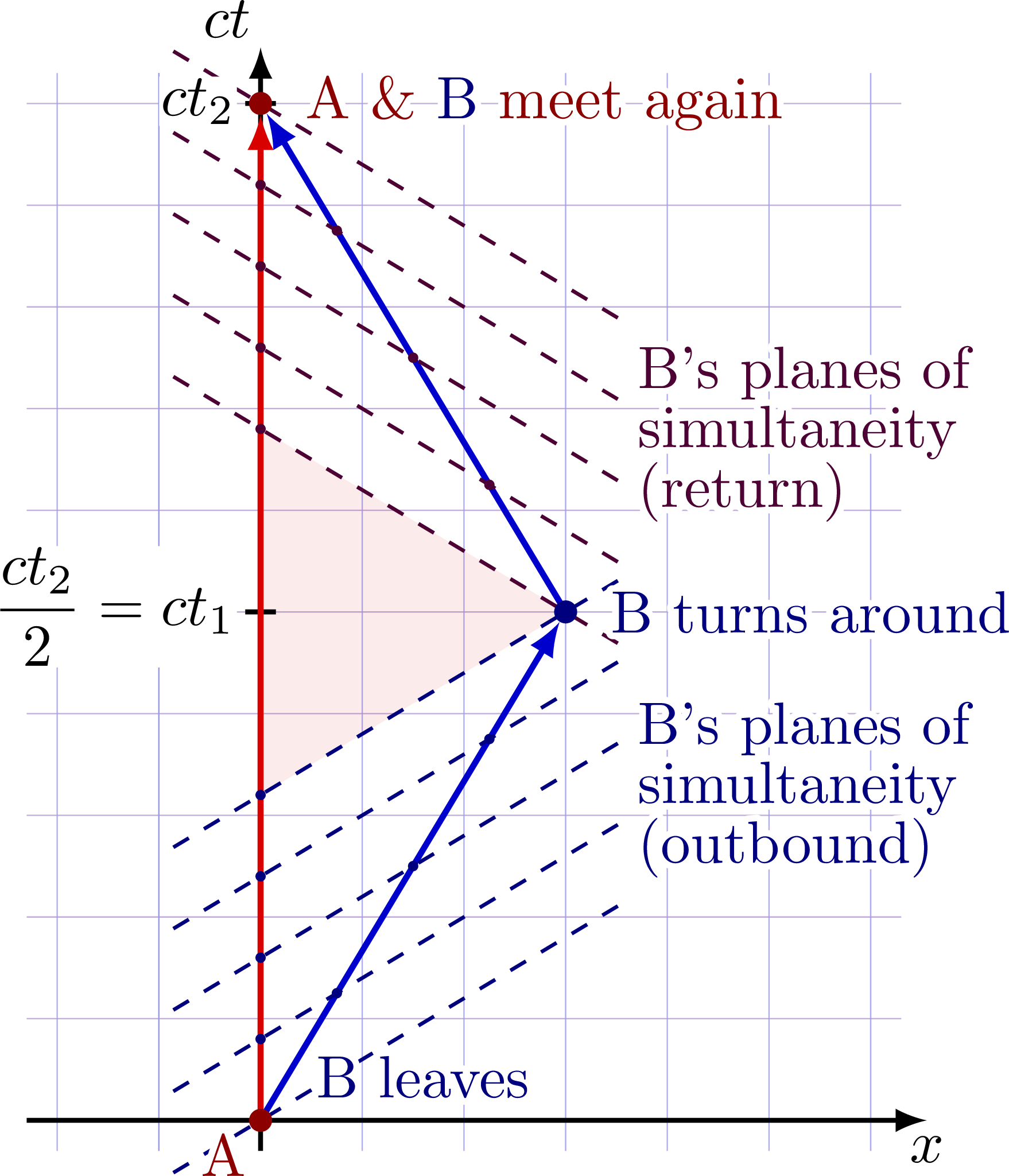
Notice the diagram is chosen such that for every 5 hours Alice measures, Bob measures 4 hours, i.e., Bob’s Lorentz factor w.r.t. Alice is γ = 5/4. One can see that before Bob turns around, the situation is symmetric. When four units of time passed in Bob frame (counted by the four blue planes of simultaneity intersecting with Alice’s word line, i.e. the time axis), just 3.2 (= 4/5*4) units of time passed in Alice’s frame (along Alice’s world line), meaning that indeed from Bob’s perspective Alice’s clock is going slower and she is aging more slowly. Only after he changes frames, and his planes of simultaneity change, is the symmetry broken.
To see more clearly what happened, and why Bob is the one who aged more slowly, it is useful to see things from Bob’s perspective. Imagine Alice sends a radio message telling Bob to turn around, shown below as a yellow photon. The message travels with the speed of light, so the photon is at a 45 degrees angle:
Let’s now look form Bob’s perspective by performing a Lorentz transformation to Bob’s rest frame. Because Bob changes frames when he turns around, we have to perform two separate transformations and paste them together. First go to Bob’s frame during the outbound trip, such that his world line coincides with the time axis, and the planes of simultaneity are horizontal:
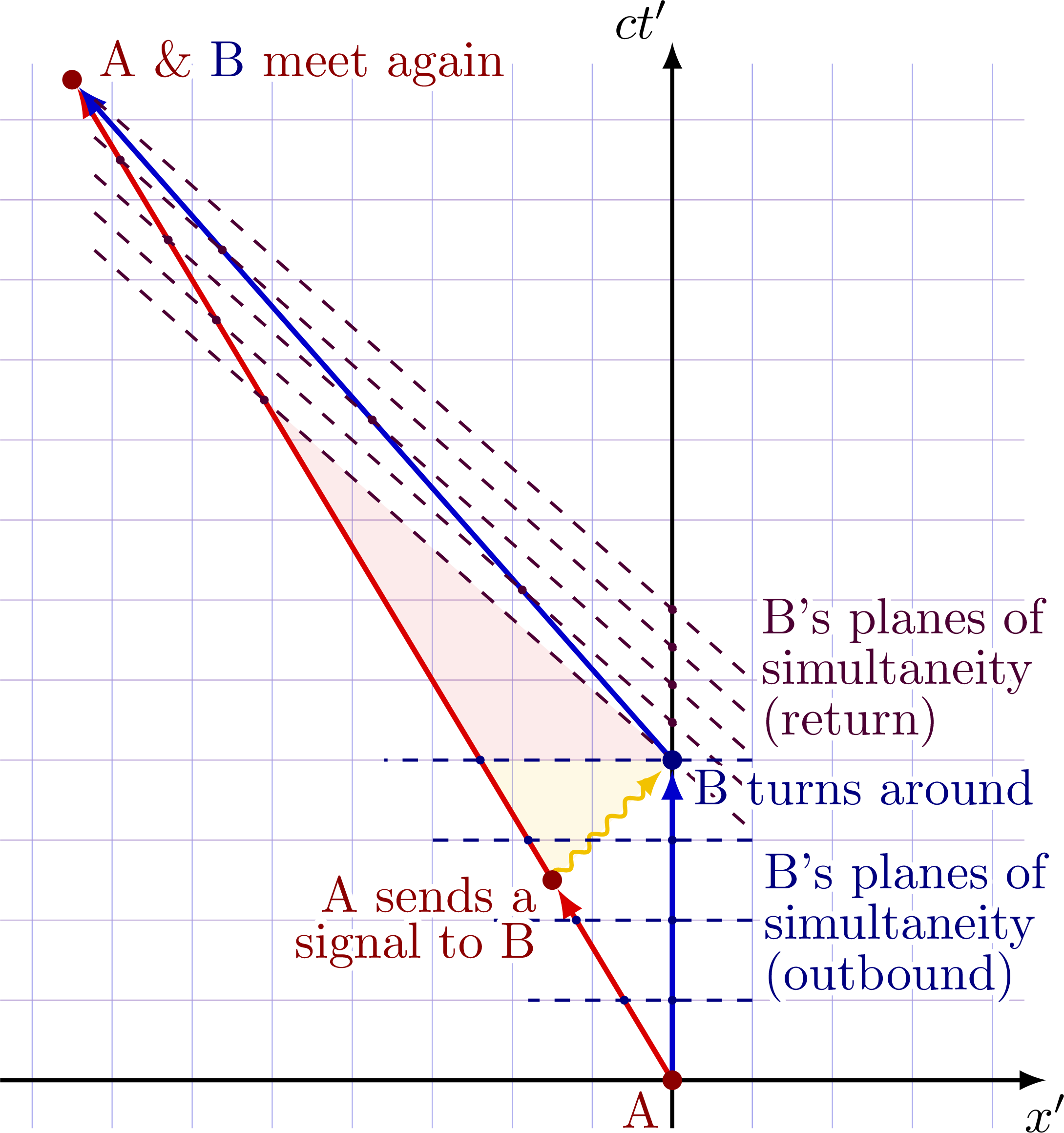
Note that Bob’s frame during the return trip travels at a relative speed of v’ = -2v/(1+β), see this Wikipedia page or this YouTube video.
Now perform a second Lorentz transform on Alice’s world line to Bob’s frame during the return trip, starting from when/where Alice had sent the message. After this transformation, we are in Bob’s full rest frame and all Bob’s planes of simultaneity are horizontal. Notice that because Bob changes frame, Alice’s world line (red vector) becomes discontinuous, and from Bob’s full rest frame, it appears that Alice “teleports” to a different spacetime point in the past. This discontinuity is because Bob changes frames, and what appears simultaneous to Bob and what is his “past”, “present”, and “future” changes. Even in Bob’s own rest frame, Alice’s world line will have a larger proper time Δt than Bob’s proper time Δt’ = Δt/γ < Δt:

Hyperbolae
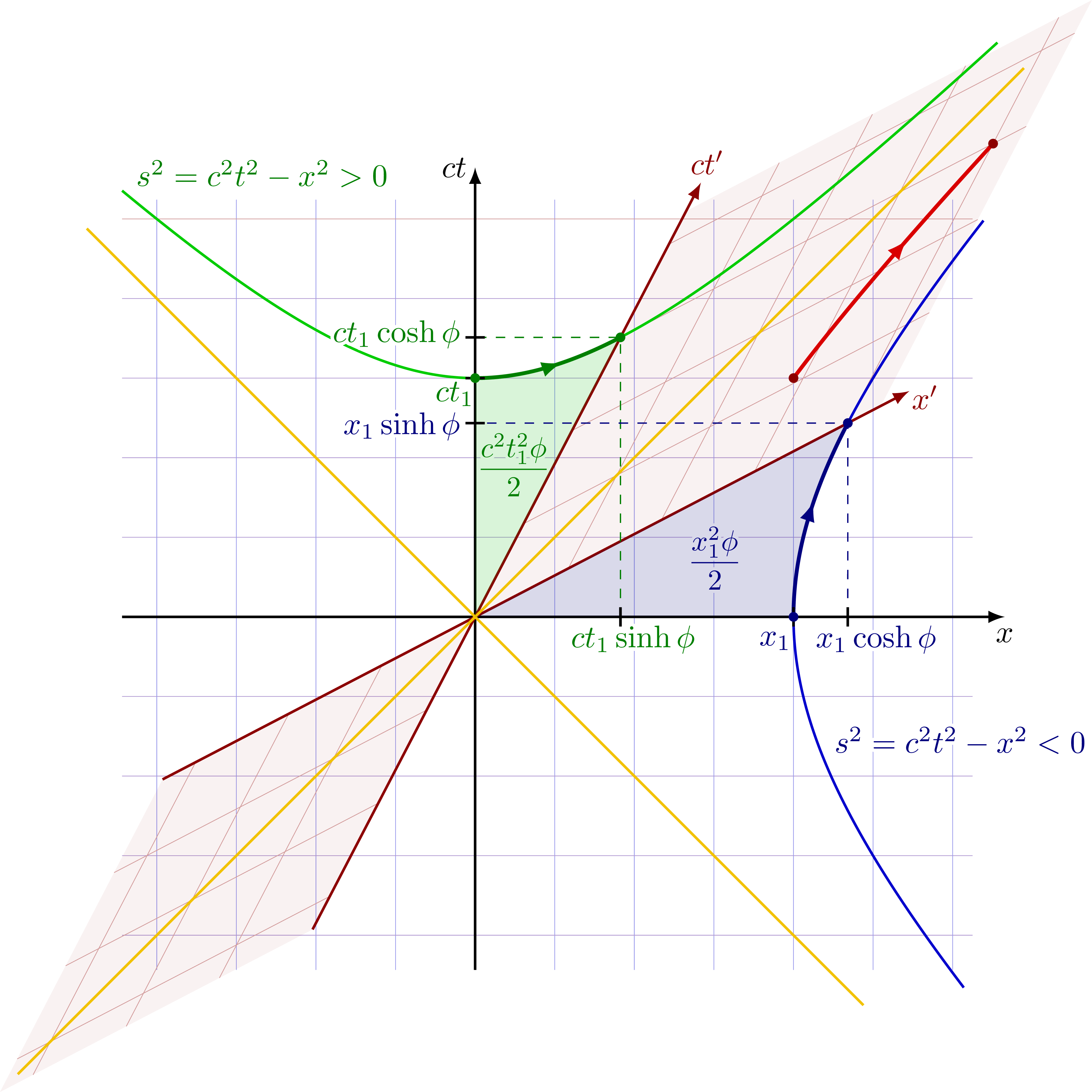
Hyperbolae in Minkowski spacetime to derive the Lorentz transformation in terms of hyperbolic functions sinh and cosh in analogy to rotation. The red point is boosted along the red hyperbola, such that its spacetime seperation from the origin remains constant.
Equations for Lorentz transformation in terms of hyperbolic functions:
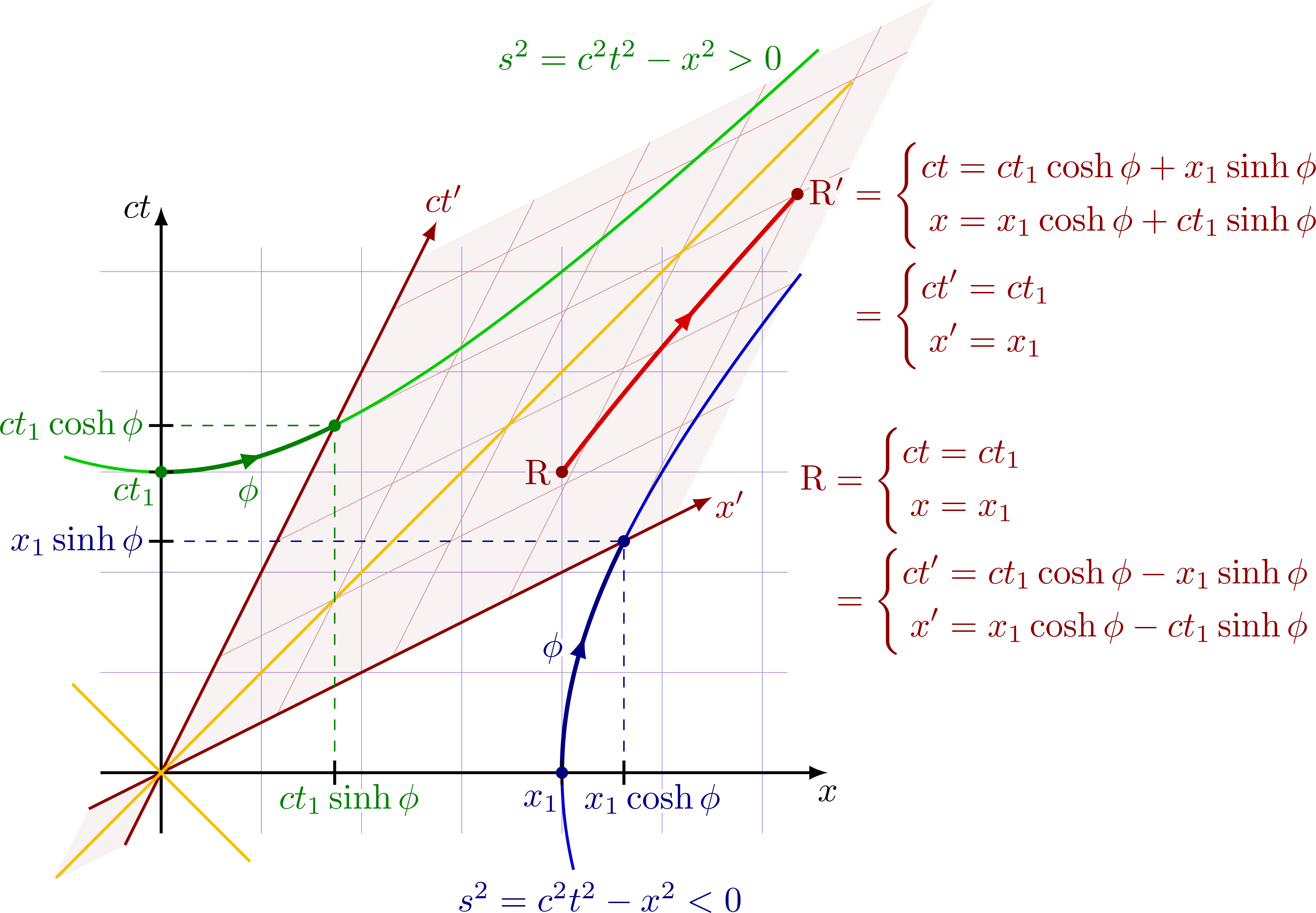
Equations for Lorentz transformation in terms of the γ factor and β = v/c:
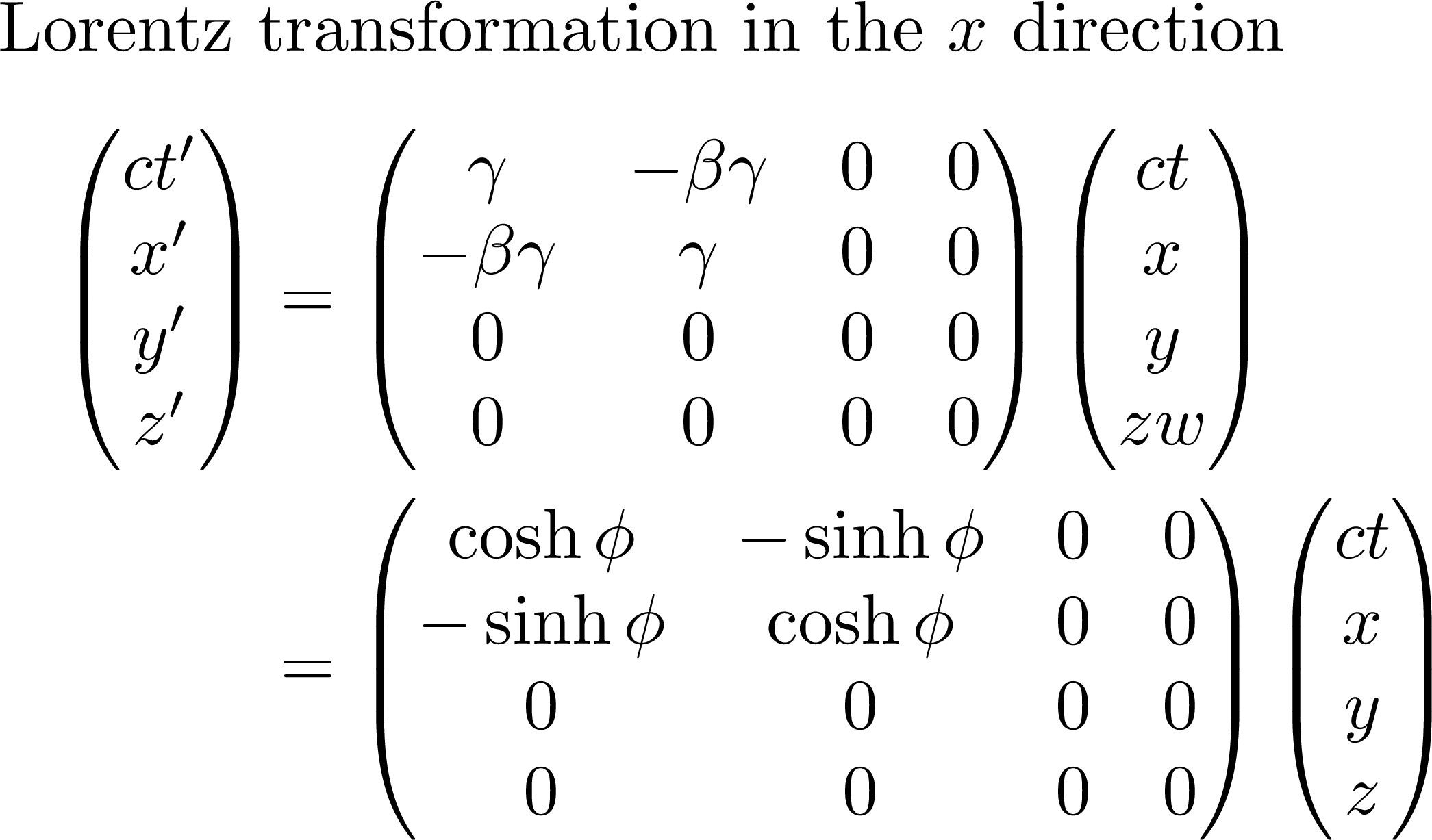
Lorentz transformation matrix with hyperbolic functions sinh and cosh in analogy to the rotation matrix. A boost is a hyperbolic rotation with rapidity 𝜑, where 𝛽 = tanh 𝜑.
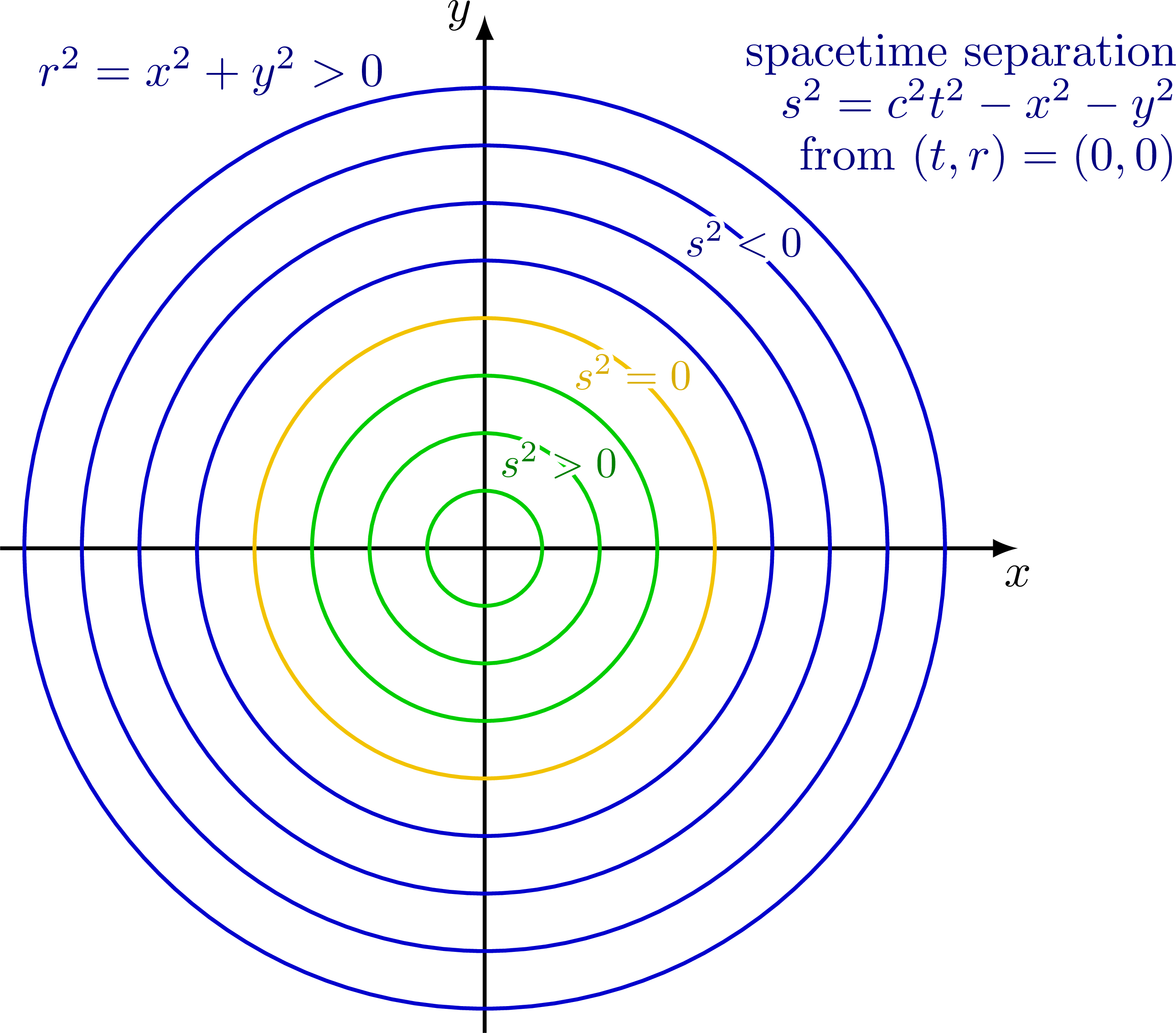
Different hyperbolae in Minkowski spacetime. All points on the same hyperbola have an equal spacetime separation s from the origin (t,x) = (0,0). A boost (i.e. a hyperbolic rotation) moves a point along such a hyperbola, and therefore preserves the spacetime distance (i.e. spacetime distance between two points are invariant under Lorentz transformations).
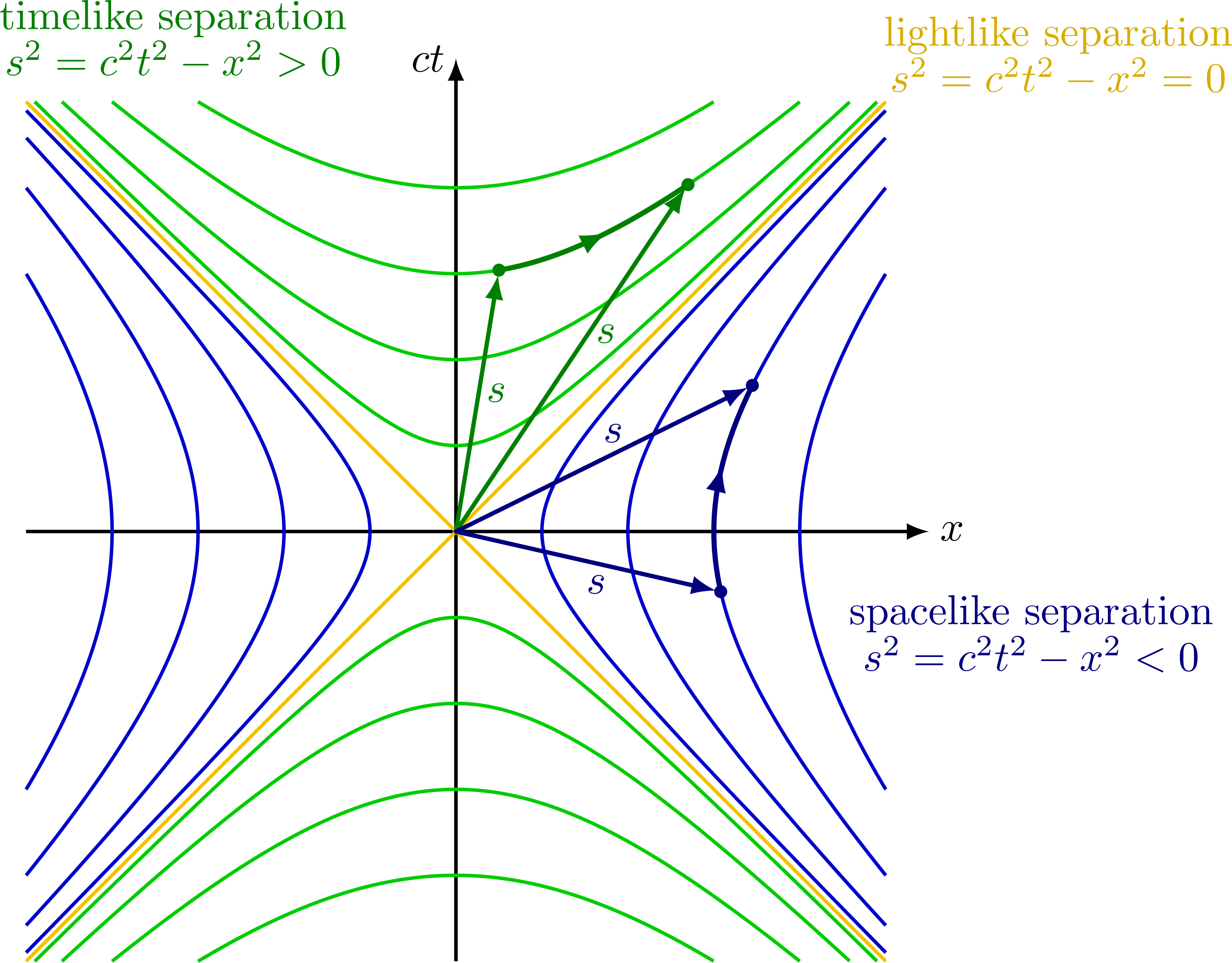
Notice that spacelike separation squared are negative, s2 < 0, so this distance will be imaginary, while timeline separations will be real.
Analogy to Euclidean rotation
Both boosts and rotations preserve the spacetime distance given by the metric ds2 = cdt2 – dx2 – dy2 – dz2. They are part of the so-called Lorentz group.
The transformation matrix for boosts in terms of hyperbolic functions looks very similar to the rotation matrix.
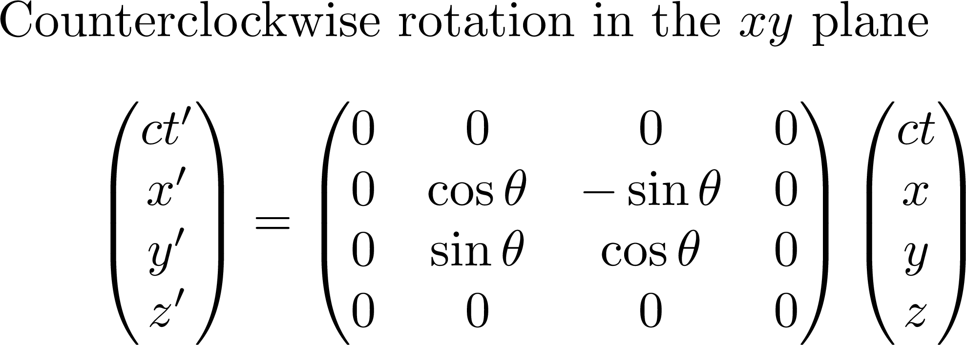
The 2D rotation matrix in the xy plane can be expressed as follows:
Spacelike slice at t = 0. All points on the same circle have the same (Euclidean) distance r to the origin. Euclidean rotations move points along the circle, and hence preserve this spacetime distance.
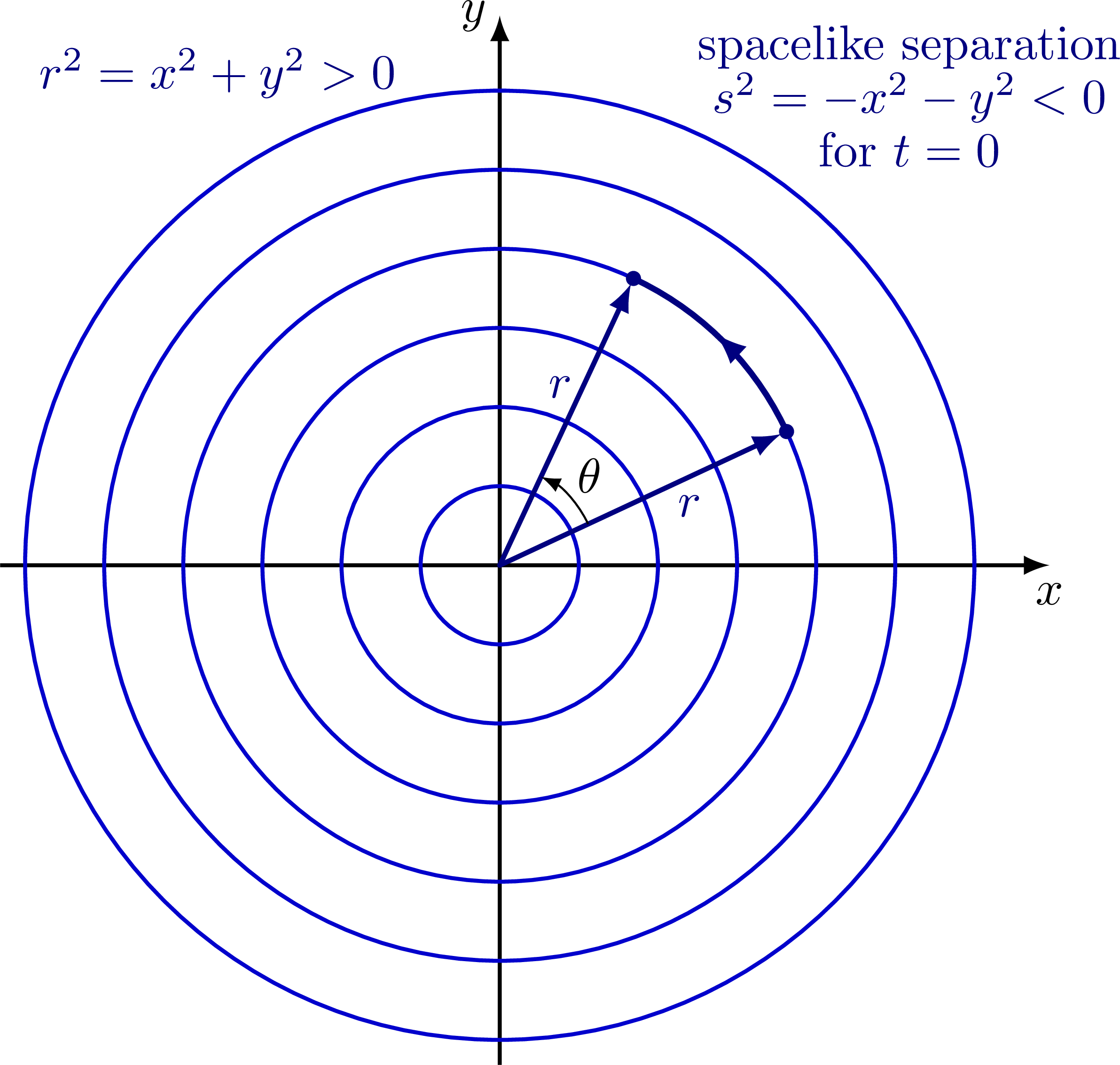
Spacelike slice to illustrate different types of separations.
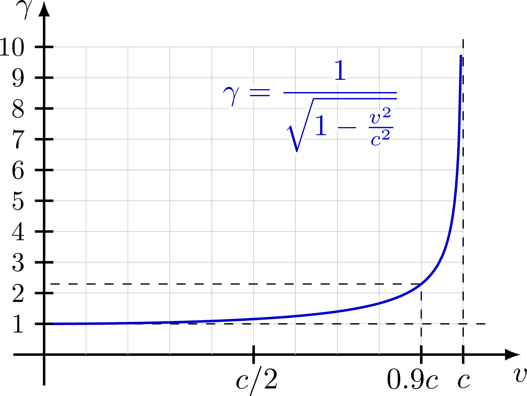
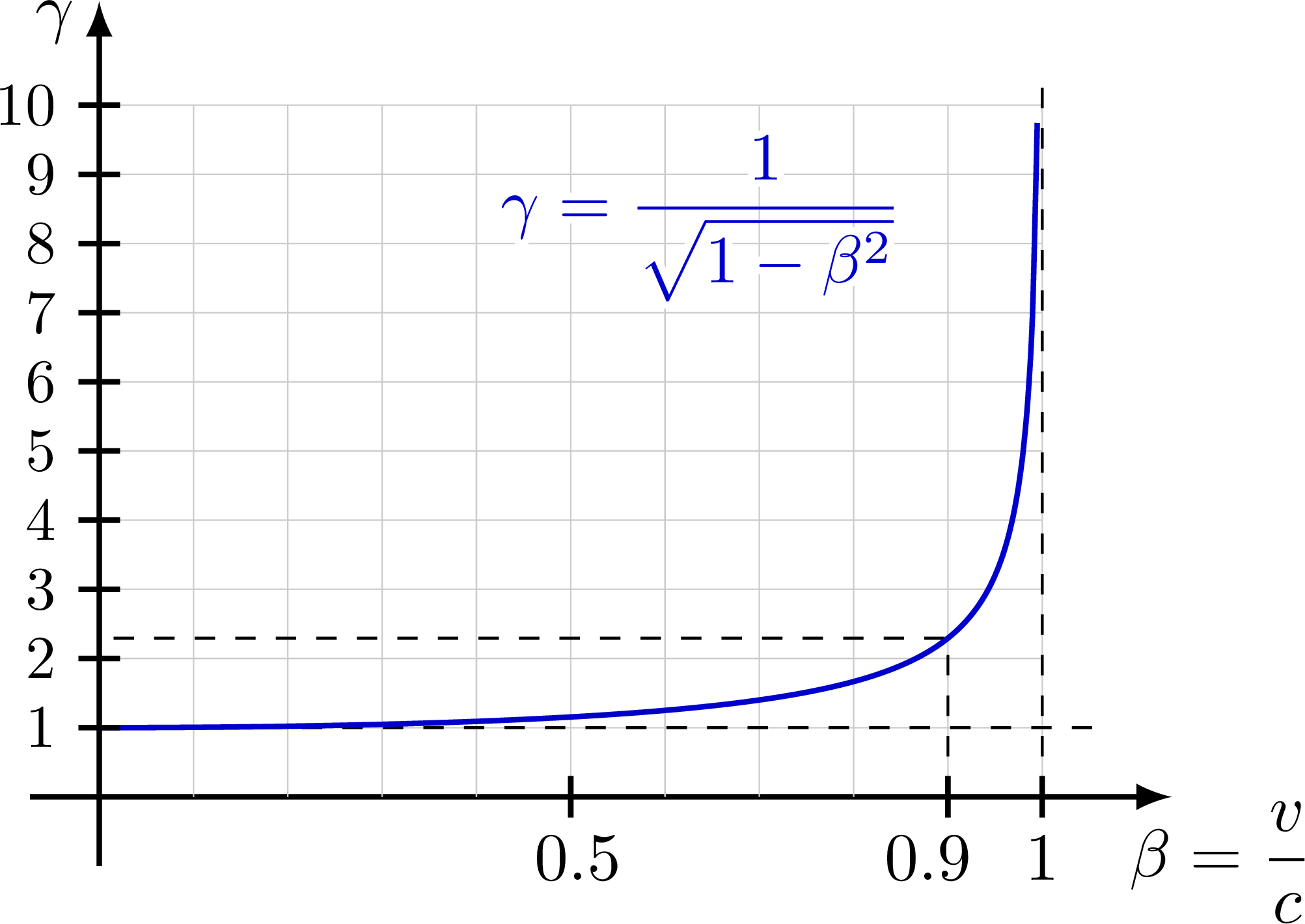
Lorentz factor
Plot of the Lorentz factor as a function of velocity v.
Plot of the Lorentz factor as a function of velocity β = v/c (i.e. in units of c).
Full code
Edit and compile if you like:
% Author: Izaak Neutelings (October 2021)
% Inspiration
% "Very special relativity - An illustrated guide", Sander Bais (2007)
% http://people.uncw.edu/hermanr/GR/Minkowski/Minkowski.pdf
\documentclass[border=3pt,tikz]{standalone}
\usepackage{amsmath} % for \text
\usepackage{etoolbox} % ifthen
\usepackage[outline]{contour} % glow around text
\usetikzlibrary{calc} % for adding up coordinates
\usetikzlibrary{decorations.markings,decorations.pathmorphing}
\usetikzlibrary{angles,quotes} % for pic (angle labels)
\usetikzlibrary{arrows.meta} % for arrow size
\usepackage{xfp} % higher precision (16 digits?)
\contourlength{1.1pt}
% COLORS
\colorlet{myred}{red!85!black}
\colorlet{mydarkred}{red!55!black}
\colorlet{mylightred}{red!85!black!12}
\colorlet{myfieldred}{mydarkred!5} % for S' background
\colorlet{myredhighlight}{myred!20} % highlights simultaneity in ladder paradox
\colorlet{myblue}{blue!80!black}
\colorlet{mydarkblue}{blue!50!black}
\colorlet{mylightblue}{blue!50!black!30}
\colorlet{mylightblue2}{myblue!10}
\colorlet{mygreen}{green!80!black}
\colorlet{mydarkgreen}{green!50!black}
\colorlet{mypurple}{blue!40!red!80!black}
\colorlet{mydarkpurple}{blue!40!red!50!black}
\colorlet{mypurple2}{blue!70!red!90!black}
\colorlet{mydarkpurple2}{blue!70!red!60!black}
\colorlet{myorange}{orange!40!yellow!95!black}
\colorlet{mydarkorange}{orange!40!yellow!85!black}
\colorlet{mybrown}{brown!20!orange!90!black}
\colorlet{mydarkbrown}{brown!20!orange!55!black}
\colorlet{mypurplehighlight}{mydarkpurple!20} % highlights simultaneity in ladder paradox
% STYLES
\tikzset{
>=latex, % for LaTeX arrow head
world line/.style={myblue!40,line width=0.2},
world line t/.style={mypurple!50!myblue!40,line width=0.2},
world line'/.style={mydarkred!40,line width=0.2},
mysmallarr/.style={-{Latex[length=3,width=2]},thin},
mydashed/.style={dash pattern=on 3 off 3},
rod/.style={mydarkbrown,draw=mydarkbrown,double=mybrown,double distance=2pt,
line width=0.2,line cap=round,shorten >=1pt,shorten <=1pt},
%rod'/.style={rod,draw=mydarkbrown!80!red!85,double=mybrown!80!red!85},
vector/.style={->,line width=1,line cap=round},
vector'/.style={vector,shorten >=1.2},
particle/.style={mygreen,line width=0.9},
photon/.style={-{Latex[length=5,width=4]},myorange,line width=0.8,decorate,
decoration={snake,amplitude=1.0,segment length=5,post length=5}}
}
\def\tick#1#2{\draw[thick] (#1) ++ (#2:0.06) --++ (#2-180:0.12)}
\def\tickp#1#2{\draw[thick,mydarkred] (#1) ++ (#2:0.06) --++ (#2-180:0.12)}
\def\Nsamples{100} % number samples in plot
\begin{document}
% SPACETIME DIAGRAM
\begin{tikzpicture}[scale=1.8]
\message{Basic spacetime diagram^^J}
\def\xmax{2}
\def\Nlines{4} % number of world lines (at constant x/t)
% WORLD LINES GRID
\message{ Making world lines...^^J}
\foreach \i [evaluate={\x=\i*0.9*\xmax/\Nlines;}] in {1,...,\Nlines}{
\message{ Running i/N=\i/\Nlines, x=\x...^^J}
\draw[world line] (-\x,-\xmax) -- (-\x,\xmax);
\draw[world line] ( \x,-\xmax) -- ( \x,\xmax);
\draw[world line t] (-\xmax,-\x) -- (\xmax,-\x);
\draw[world line t] (-\xmax, \x) -- (\xmax, \x);
}
% AXES
\draw[->,thick] (0,-\xmax) -- (0,\xmax+0.2) node[left=-1] {$ct$};
\draw[->,thick] (-\xmax,0) -- (\xmax+0.2,0) node[below=0] {$x$};
\end{tikzpicture}
% SPACETIME DIAGRAM with WORLD LINES
\begin{tikzpicture}[scale=2.0]
\message{Worldlines^^J}
\def\ymin{0.2}
\def\xmin{1.6}
\def\xmax{2}
\def\Nlines{4} % number of world lines (at constant x/t)
\pgfmathsetmacro\d{0.9*\xmax/\Nlines} % grid size
\coordinate (O) at (0,0);
\coordinate (T) at (0,\xmax+0.2);
% WORLD LINES GRID
\message{ Making world lines...^^J}
\foreach \i [evaluate={\x=\i*\d;}] in {1,...,\Nlines}{
\message{ Running i/N=\i/\Nlines, x=\x...^^J}
\draw[world line] ( \x,-\ymin) -- ( \x,\xmax);
\draw[world line t] (-\xmin, \x) -- (\xmax, \x);
}
\draw[world line] (-\d,-\ymin) -- (-\d,\xmax);
\draw[world line] (-2*\d,-\ymin) -- (-2*\d,\xmax);
\draw[world line] (-3*\d,-\ymin) -- (-3*\d,\xmax);
% AXES
\draw[->,thick] (0,-\ymin) -- (T) node[left=-1] {$ct$};
\draw[->,thick] (-\xmin,0) -- (\xmax+0.2,0) node[below=0] {$x$};
% VECTORS
\draw[vector,myorange] (O) -- (135:0.78*\xmax)
node[mydarkorange,left=6,above=-3] {\contour{white}{$x(t)=-ct$}};
\draw[vector,myblue] (O) -- ({atan(1/2)}:1.12*\xmax) %(45/2:\xmax)
node[mydarkblue,anchor=-155,outer sep=-1] {$x(t)=2ct$};
\draw[vector,myorange] (O) -- (45:1.08*\xmax)
node[mydarkorange,left=1,above right=-2] {\contour{white}{$x(t)=ct$}};
\draw[vector,mypurple] (O) -- (55:1.2*\xmax)
node[mydarkpurple,right=10,above] {\contour{white}{$x(t)=vt$}};
\draw[vector,mygreen]
(-0.10*\xmax,-0.12*\xmax) to[out=35,in=-100] (O)
to[out=80,in=-80,looseness=1.5] (0.3*\xmax,1.05*\xmax)
node[mydarkgreen,above=-3] {\contour{white}{$x(t)=v(t)t$}};
\draw[vector,myred] (O) -- (0,0.88*\xmax)
node[mydarkred,below left=0] {\contour{white}{$x(t)=0$}};
%\node[right=8,above,mydarkpurple] at (T) {$x(t)=0$};
\end{tikzpicture}
% SPACETIME DIAGRAM with TWO OBSERVERS
\begin{tikzpicture}[scale=2.0]
\message{Two observers^^J}
\def\xmin{0.2}
\def\xmax{2}
\def\R{2.03} % vector length
\def\Nlines{4} % number of world lines (at constant x/t)
\pgfmathsetmacro\d{0.9*\xmax/\Nlines} % grid size
\pgfmathsetmacro\D{2*\d} % distance between observers
\coordinate (A) at (0,0); % observer A at t=0
\coordinate (B) at (\D,0); % observer B at t=0
\coordinate (C) at (2*\d,2*\d); % point of reflection
\coordinate (T1) at (0,2*\d); % time of reflection
\coordinate (T2) at (0,4*\d); % light returning at x=0
% WORLD LINES GRID
\message{ Making world lines...^^J}
\foreach \i [evaluate={\x=\i*\d;}] in {1,...,\Nlines}{
\message{ Running i/N=\i/\Nlines, x=\x...^^J}
\draw[world line] ( \x,-\xmin) -- ( \x,\xmax);
\draw[world line t] (-\xmin, \x) -- (\xmax, \x);
}
% AXES
\draw[->,thick] (0,-\xmin) -- (0,\xmax+0.2) node[above left=-2] {$ct$};
\draw[->,thick] (-\xmin,0) -- (\xmax+0.2,0) node[below=0] {$x$};
\draw[thick,mydarkred,dashed] (T1) -- (C);
\draw[thick,mydarkred,dashed] (T2) -- (2*\d,4*\d);
% VECTORS
\draw[vector,myred] (A) --++ (0,\R)
node[mydarkred,above=-2,left=-1] {\contour{white}{$x_\mathrm{A}=0$}};
\draw[vector,mygreen] (B) --++ (0,\R)
node[mydarkgreen,left=1,above=-4] {\contour{white}{$x_\mathrm{B}'=d$}};
\draw[photon,shorten >=1] (C) -- (T2);
\fill[mydarkorange] (C) circle(0.04);
\draw[photon,shorten >=2] (A) -- (C);
\fill[mydarkred] (A) circle(0.04) node[below left=-1] {A}; % observer A
\fill[mydarkgreen] (B) circle(0.04) node[fill=white,inner sep=0.5,below=2.5] {B}; % observer B
% TICKS
\node[fill=white,inner sep=1,left=3] at (T1) {$\dfrac{ct_2}{2}=ct_1$};
\node[fill=white,inner sep=1,left=3] at (T2) {$ct_2$};
\tick{T1}{0};
\tick{T2}{0};
\end{tikzpicture}
% SPACETIME DIAGRAM with TWO MOVING OBSERVERS to show simultaneity
\begin{tikzpicture}[scale=2.0]
\message{Two moving observers^^J}
\def\xmin{0.2}
\def\xmax{2}
\def\R{2.3} % vector length
\def\Nlines{4} % number of world lines (at constant x/t)
\pgfmathsetmacro\ang{73} % angle between ct and ct' axes
\pgfmathsetmacro\d{0.9*\xmax/\Nlines} % grid size
\pgfmathsetmacro\D{2*\d} % distance between observers
\coordinate (A) at (0,0); % observer A at t=0
\coordinate (B) at (\D,0); % observer B at t=0
\coordinate (C) at (45:{\D*sqrt(2)/(1-cot(\ang))}); % point of reflection
%\coordinate (T1) at (\ang:{2*\d/sin(\ang)/sqrt(1-cot(\ang)^2)}); % time of reflection
\coordinate (T1) at (\ang:{\D*sqrt(cot(\ang)^2+1)/(1-cot(\ang)^2)}); % time of reflection
\coordinate (T2) at (\ang:{2*\D*sqrt(cot(\ang)^2+1)/(1-cot(\ang)^2)}); % time of reflection
% WORLD LINES GRID
\message{ Making world lines...^^J}
\foreach \i [evaluate={\x=\i*\d;}] in {1,...,\Nlines}{
\message{ Running i/N=\i/\Nlines, x=\x...^^J}
\draw[world line] ( \x,-\xmin) -- ( \x,\xmax);
\draw[world line t] (-\xmin, \x) -- (\xmax, \x);
}
% AXES
\draw[->,thick] (0,-\xmin) -- (0,\xmax+0.2) node[above left=-2] {$ct$};
\draw[->,thick] (-\xmin,0) -- (\xmax+0.2,0) node[below=0] {$x$};
\draw[->,thick,mydarkred,dashed] (A) -- (90-\ang:\xmax) node[above=1,right=-1] {$x$}; %_\mathrm{A}'
\draw[->,thick,mydarkred,dashed] (T1) --++ (90-\ang:\xmax);
% VECTORS
\draw[vector,myred] (A) --++ (\ang:\R)
node[mydarkred,left=1,above=-2] {$x_\mathrm{A}=vt$};
\draw[vector,mygreen] (B) --++ (\ang:\R)
node[mydarkgreen,right=6,above=-2] {$x_\mathrm{B}=d+vt$};
\draw[photon,shorten >=1] (C) --++ (135:{\D*sqrt(2)/(1+cot(\ang))});
\fill[mydarkorange] (C) circle(0.04);
\draw[photon,shorten >=2] (A) -- (C);
\fill[mydarkred] (A) circle(0.04) node[below left=-1] {A}; % observer A
\fill[mydarkgreen] (B) circle(0.04) node[fill=white,inner sep=0.5,below=2.5] {B}; % observer B
% TICKS
%\node[fill=white,inner sep=1,left=3] at (T1) {$\dfrac{ct_2}{2}=ct_1$};
%\node[fill=white,inner sep=1,left=3] at (T2) {$ct_2$};
\tickp{T1}{90-\ang} node[left=-4] {\contour{white}{$\dfrac{ct_2'}{2}=ct_1'$}};
\tickp{T2}{90-\ang} node[left=-3] {\contour{white}{$ct_2'$}};
\end{tikzpicture}
% SPACETIME DIAGRAM - LIGHT CONE
\begin{tikzpicture}[scale=1.8]
\message{Light cone^^J}
\def\xmax{2}
\def\xmaxp{2.2} % maximum of rotated axis
\def\Nlines{5} % number of world lines (at constant x/t)
\pgfmathsetmacro\d{0.9*\xmax/\Nlines} % grid size
\pgfmathsetmacro\ang{atan(1/3)} % angle between x and x' axes
\coordinate (O) at (0,0);
\coordinate (X) at (\xmax+0.2,0);
\coordinate (T) at (0,\xmax+0.2);
% WORLD LINE GRID
\message{ Making world lines...^^J}
\foreach \i [evaluate={\x=\i*\d;}] in {1,...,\Nlines}{
\message{ Running i/N=\i/\Nlines, x=\x...^^J}
\draw[world line] (-\x,-\xmax) -- (-\x,\xmax);
\draw[world line] ( \x,-\xmax) -- ( \x,\xmax);
\draw[world line t] (-\xmax,-\x) -- (\xmax,-\x);
\draw[world line t] (-\xmax, \x) -- (\xmax, \x);
}
% AXES
\draw[->,thick] (0,-\xmax) -- (T) node[left=-1] {$ct$};
\draw[->,thick] (-\xmax,0) -- (X) node[below=0] {$x$};
% LABELS
\draw pic[->,"$45^\circ$",draw=black,angle radius=23,angle eccentricity=1.38] {angle = X--O--C};
\node[mydarkorange,above right] at (0.1*\xmax,\xmax) {future light cone};
\node[mydarkorange,below] at (0,-\xmax) {past light cone};
% FILLS
\fill[myblue,opacity=0.05] % SPACELIKE
(\xmax,\xmax) -- (-\xmax,-\xmax) -- (-\xmax,\xmax) -- (\xmax,-\xmax) -- cycle;
\fill[myorange,opacity=0.05] % TIMELIKE
(\xmax,\xmax) -- (-\xmax,\xmax) -- (\xmax,-\xmax) -- (-\xmax,-\xmax) -- cycle;
\node[mydarkblue,right,align=center] at (-\xmax,0.18*\xmax)
{\contour{myblue!5}{spacelike}\\[-2]\contour{myblue!5}{region}};
\node[mydarkblue,left,align=center] at (\xmax,0.18*\xmax)
{\contour{myblue!5}{spacelike}\\[-2]\contour{myblue!5}{region}};
\node[mydarkorange,align=center] at (-0.22*\xmax,0.67*\xmax)
{\contour{myorange!5}{timelike}\\[-2]\contour{myorange!5}{region}};
\node[mydarkorange,align=center] at (0.22*\xmax,-0.67*\xmax)
{\contour{myorange!5}{timelike}\\[-2]\contour{myorange!5}{region}};
% PHOTON
\draw[photon] ( \xmax,-\xmax) -- ( 0.02*\xmax,-0.02*\xmax);
\draw[photon] (-\xmax,-\xmax) -- (-0.02*\xmax,-0.02*\xmax);
\draw[photon] ( 0.02*\xmax,0.02*\xmax) -- ( \xmax,\xmax)
node[mydarkorange,above right] {$x=ct$};
\draw[photon] (-0.02*\xmax,0.02*\xmax) -- (-\xmax,\xmax);
% PARTICLE WORLDLINE
\draw[particle,decoration={markings,mark=at position 0.27 with {\arrow{latex}},
mark=at position 0.76 with {\arrow{latex}}},postaction={decorate}]
(-0.5*\xmax,-\xmax) to[out=80,in=-110] (O) to[out=70,in=-100] (0.45*\xmax,\xmax);
\fill[mydarkgreen] (O) circle(0.04); % event
\end{tikzpicture}
% SPACETIME DIAGRAM - VECTORS
\begin{tikzpicture}[scale=1.8]
\message{Vectors^^J}
\def\xmax{2}
\def\xmaxp{2.2} % maximum of rotated axis
\def\Nlines{5} % number of world lines (at constant x/t)
\pgfmathsetmacro\d{0.9*\xmax/\Nlines} % grid size
\pgfmathsetmacro\ang{atan(1/3)} % angle between x and x' axes
\coordinate (O) at (0,0);
\coordinate (X) at (\xmax+0.2,0);
\coordinate (T) at (0,\xmax+0.2);
% WORLD LINE GRID
\message{ Making world lines...^^J}
\foreach \i [evaluate={\x=\i*\d;}] in {1,...,\Nlines}{
\message{ Running i/N=\i/\Nlines, x=\x...^^J}
\draw[world line] (-\x,-\xmax) -- (-\x,\xmax);
\draw[world line] ( \x,-\xmax) -- ( \x,\xmax);
\draw[world line t] (-\xmax,-\x) -- (\xmax,-\x);
\draw[world line t] (-\xmax, \x) -- (\xmax, \x);
}
% FILLS
\fill[myblue,opacity=0.05] % SPACELIKE
(\xmax,\xmax) -- (-\xmax,-\xmax) -- (-\xmax,\xmax) -- (\xmax,-\xmax) -- cycle;
\fill[mygreen,opacity=0.05] % TIMELIKE
(\xmax,\xmax) -- (-\xmax,\xmax) -- (\xmax,-\xmax) -- (-\xmax,-\xmax) -- cycle;
% AXES
\draw[->,thick] (0,-\xmax) -- (T) node[left=-1] {$ct$};
\draw[->,thick] (-\xmax,0) -- (X) node[below=0] {$x$};
% VECTORS
\draw[vector,mygreen] (O) --++ (68:0.79*\xmax)
node[right=4,above=-1,align=center]
{\contour{mygreen!5}{timelike vector}\\[-1]
\contour{mygreen!5}{$s^2=c^2t^2-x^2>0$}};
\draw[vector,myblue] (O) --++ (28:0.63*\xmax)
node[below=7,right=-22,align=center]
{\contour{myblue!5}{spacelike}\\[-2]
\contour{myblue!5}{vector}\\[-1]
\contour{myblue!5}{$s^2=c^2t^2-x^2<0$}};
\draw[vector,mygreen,<->] (-2*\d,-\d) --++ (-2*\d,3.5*\d)
node[pos=0.8,below left=-2,align=right]
{\contour{myblue!5}{timelike}\\[-2]
\contour{myblue!5}{separation}\\[-1]
\contour{myblue!5}{$\Delta s^2>0$}};
\draw[vector,myblue,<->] (2*\d,-\d) --++ (3*\d,-2*\d)
node[pos=0.4,above right=-2,align=left]
{\contour{myblue!5}{spacelike}\\[-2]
\contour{myblue!5}{separation}\\[-1]
\contour{myblue!5}{$\Delta s^2<0$}};
\draw[vector,myorange,<->] (2*\d,-3*\d) --++ (2*\d,-2*\d)
node[pos=0.45,below left=-4,align=center]
{\contour{mygreen!5}{lightlike}\\[-2]
\contour{mygreen!5}{separation}\\[-1]
\contour{mygreen!5}{$\Delta s^2 = 0$}};
% PHOTON
\draw[photon] ( \xmax,-\xmax) -- ( 0.02*\xmax,-0.02*\xmax);
\draw[photon] (-\xmax,-\xmax) -- (-0.02*\xmax,-0.02*\xmax);
\draw[photon] ( 0.02*\xmax,0.02*\xmax) -- ( \xmax,\xmax)
node[mydarkorange,above=-1,align=center] {lightlike vector\\[-2]$s^2=c^2t^2+x^2=0$};
\draw[photon] (-0.02*\xmax,0.02*\xmax) -- (-\xmax,\xmax);
\end{tikzpicture}
% SPACETIME DIAGRAM - OVERLAPPING LIGHT CONES
\begin{tikzpicture}[scale=1.8]
\message{Overlapping light cones^^J}
\def\xmax{2}
\def\ext{4*\d} % extension x axis
\def\xmaxp{2.2} % maximum of rotated axis
\def\Nlines{5} % number of world lines (at constant x/t)
\pgfmathsetmacro\d{0.9*\xmax/\Nlines} % grid size
\pgfmathsetmacro\ang{atan(1/3)} % angle between x and x' axes
\coordinate (O) at (0,0);
\coordinate (X) at (\xmax+\ext+0.2,0);
\coordinate (T) at (0,\xmax+0.2);
\coordinate (B) at (4*\d,0); % event B
% WORLD LINE GRID
\message{ Making world lines...^^J}
\foreach \i [evaluate={\x=\i*\d;}] in {1,...,\Nlines}{
\message{ Running i/N=\i/\Nlines, x=\x...^^J}
\draw[world line] (-\x,-\xmax) -- (-\x,\xmax);
\draw[world line] ( \x,-\xmax) -- ( \x,\xmax);
\draw[world line t] (-\xmax,-\x) -- (\xmax+\ext,-\x);
\draw[world line t] (-\xmax, \x) -- (\xmax+\ext, \x);
}
\foreach \i [evaluate={\x=(\Nlines+\i)*\d;}] in {1,...,4}{
\message{ Running i/N=\i/\Nlines, x=\x...^^J}
\draw[world line] (\x,-\xmax) -- ( \x,\xmax);
}
% AXES
\draw[->,thick] (0,-\xmax) -- (T) node[left=-1] {${\color{mydarkred}ct'}=ct$};
\draw[->,thick] (-\xmax,0) -- (X) node[below=0] {$x$};
% LIGHT CONES
\begin{scope}[shift={(B)}]
\fill[myorange!70!red,opacity=0.09]
(0,0) -- (\xmax,\xmax) -- (-\xmax,\xmax) -- (\xmax,-\xmax) -- (-\xmax,-\xmax) -- cycle;
\end{scope}
\fill[myorange!70!green,opacity=0.09]
(O) -- (\xmax,\xmax) -- (-\xmax,\xmax) -- (\xmax,-\xmax) -- (-\xmax,-\xmax) -- cycle;
% PHOTONS
\draw[photon] (135:0.1) -- (135:0.4*\xmax);
\draw[photon] (45:0.1) -- (45:0.4*\xmax);
\draw[photon] (B)++(135:0.1) --++ (135:0.4*\xmax);
\draw[photon] (B)++(45:0.1) --++ (45:0.4*\xmax);
%\draw[photon] (0.05,0.05) -- ( \xmax,\xmax)
% node[mydarkorange,above right] {$x=ct$};
% PARTICLE WORLDLINES
\draw[particle,decoration={markings,mark=at position 0.27 with {\arrow{latex}},
mark=at position 0.76 with {\arrow{latex}}},postaction={decorate}]
(-0.5*\xmax,-\xmax) to[out=80,in=-110] (O) to[out=70,in=-100] (0.45*\xmax,\xmax);
\draw[particle,myred,decoration={markings,mark=at position 0.27 with {\arrow{latex}},
mark=at position 0.74 with {\arrow{latex}}},postaction={decorate}]
(0.84*\xmax,-\xmax) to[out=95,in=-80] (B) to[out=100,in=-76] (0.49*\xmax,\xmax);
% EVENTS
\fill[mydarkgreen] (O) circle(0.04); % event A
\fill[mydarkred] (B) circle(0.04); % event B
\end{tikzpicture}
% SPACETIME DIAGRAM - OVERLAPPING LIGHT CONES with boosted frame
\begin{tikzpicture}[scale=1.8]
\message{Lorentz boost^^J}
\def\xmax{2}
\def\xmaxp{2.2} % maximum of rotated axis
\def\ext{4*\d} % extension x axis
\def\Nlines{5} % number of world lines (at constant x/t)
\pgfmathsetmacro\ang{atan(1/4)} % angle between x and x' axes
\pgfmathsetmacro\d{0.9*\xmax/\Nlines} % grid size
\pgfmathsetmacro\D{\d/cos(\ang)/sqrt(1-tan(\ang)^2)} % grid size, boosted
\coordinate (O) at (0,0);
\coordinate (X) at (\xmax+\ext+0.2,0);
\coordinate (T) at (0,\xmax+0.2);
\coordinate (X') at (\ang:\xmaxp+0.2);
\coordinate (T') at (90-\ang:\xmaxp+0.2);
\coordinate (B) at ($(\ang:3*\D)+(90-\ang:1*\D)$); % event
% WORLD LINE GRID
\message{ Making world lines...^^J}
\foreach \i [evaluate={\x=\i*\d;}] in {1,...,\Nlines}{
\message{ Running i/N=\i/\Nlines, x=\x...^^J}
\draw[world line] (-\x,-\xmax) -- (-\x,\xmax);
\draw[world line] ( \x,-\xmax) -- ( \x,\xmax);
\draw[world line t] (-\xmax,-\x) -- (\xmax+\ext,-\x);
\draw[world line t] (-\xmax, \x) -- (\xmax+\ext, \x);
}
\foreach \i [evaluate={\x=(\Nlines+\i)*\d;}] in {1,...,4}{
\message{ Running i/N=\i/\Nlines, x=\x...^^J}
\draw[world line] (\x,-\xmax) -- ( \x,\xmax);
}
% BOOSTED WORLD LINE GRID
\message{ Making world lines for boosted frame...^^J}
\fill[mydarkred,opacity=0.05]
(O) --++ (\ang:\xmaxp) --++ (90-\ang:\xmaxp) --++ (\ang:-\xmaxp) -- cycle;
\fill[mydarkred,opacity=0.05]
(O) --++ (\ang:-\xmaxp) --++ (90-\ang:-\xmaxp) --++ (\ang:\xmaxp) -- cycle;
\foreach \i [evaluate={\x=\i*\D;}] in {1,...,\Nlines}{
\message{ Running i/N=\i/\Nlines, x=\x...^^J}
\draw[world line'] (\ang:-\x) --++ (90-\ang:-\xmaxp);
\draw[world line'] (90-\ang:-\x) --++ (\ang:-\xmaxp);
\draw[world line'] (\ang:\x) --++ (90-\ang:\xmaxp);
\draw[world line'] (90-\ang:\x) --++ (\ang:\xmaxp);
}
% LIGHT CONES
\begin{scope}
\clip (-\xmax,-\xmax) rectangle (\xmax+\ext,\xmax);
\fill[myorange!70!red,opacity=0.09,shift={(B)}]
(0,0) -- (\xmax,\xmax) -- (-\xmax,\xmax) -- (2*\xmax,-2*\xmax) -- (-2*\xmax,-2*\xmax) -- cycle;
\end{scope}
\fill[myorange!70!green,opacity=0.09]
(O) -- (\xmax,\xmax) -- (-\xmax,\xmax) -- (\xmax,-\xmax) -- (-\xmax,-\xmax) -- cycle;
% PHOTONS
\draw[photon] (135:0.12) -- (135:0.4*\xmax);
\draw[photon] (45:0.12) -- (45:0.4*\xmax);
\draw[photon] (B)++(135:0.12) --++ (135:0.4*\xmax);
\draw[photon] (B)++(45:0.12) --++ (45:0.4*\xmax);
% AXES
\draw[->,thick] (0,-\xmax) -- (T) node[left=-1] {$ct$};
\draw[->,thick] (-\xmax,0) -- (X) node[below=0] {$x$};
\draw[->,thick,mydarkred] (90-\ang:-\xmaxp) -- (T')
node[right=5,above=-1] {$ct' = \gamma\left(ct-\beta x\right)$};
\draw[->,thick,mydarkred] (\ang:-\xmaxp) -- (X') node[right=-1] {$x' = \gamma(x-vt)$};
% EVENTS
\fill[mydarkgreen] (O) circle(0.05); % event A
\fill[mydarkred] (B) circle(0.05); % event B
\end{tikzpicture}
% SPACETIME DIAGRAM - EUCLIDEAN ROTATION
\begin{tikzpicture}[scale=1.8]
\message{Rotation^^J}
\def\xmax{2}
\def\xmaxp{2.1} % maximum of rotated axis
\def\Nlines{5} % number of world lines (at constant x/t)
\pgfmathsetmacro\ang{20} % angle between x and x' axes
\pgfmathsetmacro\d{0.9*\xmax/\Nlines} % grid size
\coordinate (O) at (0,0);
\coordinate (X) at (\xmax+0.2,0);
\coordinate (T) at (0,{(1+0.5*sin(\ang))*\xmax+0.2});
\coordinate (X') at (\ang:\xmaxp+0.2);
\coordinate (T') at (90+\ang:\xmaxp+0.2);
% WORLD LINE GRID
\message{ Making world lines...^^J}
\foreach \i [evaluate={\x=\i*\d;}] in {1,...,\Nlines}{
\message{ Running i/N=\i/\Nlines, x=\x...^^J}
\draw[world line] (-\x,-\xmax) -- (-\x,\xmax);
\draw[world line] ( \x,-\xmax) -- ( \x,\xmax);
\draw[world line t] (-\xmax,-\x) -- (\xmax,-\x);
\draw[world line t] (-\xmax, \x) -- (\xmax, \x);
}
% BOOSTED WORLD LINE GRID
\message{ Making world lines for boosted frame...^^J}
\fill[mydarkred,opacity=0.05]
(O) --++ (\ang:\xmaxp) --++ (90+\ang:\xmaxp) --++ (\ang:-\xmaxp) -- cycle;
\fill[mydarkred,opacity=0.05]
(O) --++ (\ang:-\xmaxp) --++ (90+\ang:-\xmaxp) --++ (\ang:\xmaxp) -- cycle;
\foreach \i [evaluate={\x=\i*\d;}] in {1,...,\Nlines}{
\message{ Running i/N=\i/\Nlines, x=\x...^^J}
\draw[world line'] (\ang:-\x) --++ (90+\ang:-\xmaxp);
\draw[world line'] (90+\ang:-\x) --++ (\ang:-\xmaxp);
\draw[world line'] (\ang:\x) --++ (90+\ang:\xmaxp);
\draw[world line'] (90+\ang:\x) --++ (\ang:\xmaxp);
}
% AXES
\draw[->,thick] (0,-\xmax) -- (T) node[left=-1] {$y$};
\draw[->,thick] (-\xmax,0) -- (X) node[below=0] {$x$};
\draw[->,thick,mydarkred] (90+\ang:-\xmaxp) -- (T')
node[left=13,above=-1] {$y'=\cos\theta\,y-\sin\theta\,x$};
\draw[->,thick,mydarkred] (\ang:-\xmaxp) -- (X')
node[above=7,right=-11] {$x'=\cos\theta\,x+\sin\theta\,y$};
% ANGLES
\draw pic[->,"$\theta$",draw=black,angle radius=34,angle eccentricity=1.2] {angle = X--O--X'};
\draw pic[->,"$\theta$",draw=black,angle radius=35,angle eccentricity=1.2] {angle = T--O--T'};
\end{tikzpicture}
% SPACETIME DIAGRAM - GALILEAN TRANSFORMATION
\begin{tikzpicture}[scale=1.8]
\message{Galilean transformation^^J}
\def\xmax{2}
\def\xmaxp{2.1} % maximum of rotated axis
\def\Nlines{4} % number of world lines (at constant x/t)
\pgfmathsetmacro\d{0.9*\xmax/\Nlines} % grid size
\pgfmathsetmacro\ang{atan(1/3)} % angle
\coordinate (O) at (0,0);
\coordinate (X) at (\xmax+0.2,0);
\coordinate (T) at (0,\xmax+0.2);
\coordinate (X') at (\ang:\xmaxp+0.2);
\coordinate (T') at (90-\ang:\xmaxp+0.2);
% WORLD LINES GRID
\message{ Making world lines...^^J}
\foreach \i [evaluate={\x=\i*\d;}] in {1,...,\Nlines}{
\message{ Running i/N=\i/\Nlines, x=\x...^^J}
\draw[world line] (-\x,-\xmax) -- (-\x,\xmax);
\draw[world line] ( \x,-\xmax) -- ( \x,\xmax);
\draw[world line t] ({-\xmax-tan(\ang)*\x},-\x) -- (\xmax,-\x);
\draw[world line t] (-\xmax,\x) -- ({\xmax+tan(\ang)*\x},\x);
}
% AXES
\draw[->,thick] (0,-\xmax) -- (T) node[left=0] {$ct$};
\draw[->,thick] (-\xmax,0) -- (X) node[right=6,below=-1] {$x={\color{mydarkred}x'}$};
\draw[->,thick,mydarkred] (90-\ang:-\xmaxp) -- (T')
node[left=-1] {$ct'$}
node[right=2,below right=-2] {$x = vt$};
% WORLD LINES GRID - BOOSTED
\message{ Making world lines, boosted...^^J}
\fill[mydarkred,opacity=0.05]
(O) --++ (90-\ang:\xmax) --++ (\xmax,0) --++ (90-\ang:-\xmax) -- cycle;
\fill[mydarkred,opacity=0.05]
(O) --++ (90-\ang:-\xmax) --++ (-\xmax,0) --++ (90-\ang:\xmax) -- cycle;
\foreach \i [evaluate={\x=\i*\d;}] in {1,...,\Nlines}{
\message{ Running i/N=\i/\Nlines, x=\x...^^J}
\draw[world line'] (\x,0) --++ (90-\ang:\xmax);
\draw[world line'] (-\x,0) --++ (90-\ang:-\xmax);
}
\draw pic[<-,"$\theta$",draw=black,angle radius=34,angle eccentricity=1.2] {angle = T'--O--T};
\end{tikzpicture}
% SPACETIME DIAGRAM - LORENTZ BOOST
\begin{tikzpicture}[scale=1.8]
\message{Lorentz boost^^J}
\def\xmax{2}
\def\xmaxp{2.2} % maximum of rotated axis
\def\Nlines{5} % number of world lines (at constant x/t)
\pgfmathsetmacro\ang{atan(1/3)} % angle between x and x' axes
\pgfmathsetmacro\d{0.9*\xmax/\Nlines} % grid size
\pgfmathsetmacro\D{\d/cos(\ang)/sqrt(1-tan(\ang)^2)} % grid size, boosted
\coordinate (O) at (0,0);
\coordinate (X) at (\xmax+0.2,0);
\coordinate (T) at (0,\xmax+0.2);
\coordinate (X') at (\ang:\xmaxp+0.2);
\coordinate (T') at (90-\ang:\xmaxp+0.2);
% WORLD LINE GRID
\message{ Making world lines...^^J}
\foreach \i [evaluate={\x=\i*\d;}] in {1,...,\Nlines}{
\message{ Running i/N=\i/\Nlines, x=\x...^^J}
\draw[world line] (-\x,-\xmax) -- (-\x,\xmax);
\draw[world line] ( \x,-\xmax) -- ( \x,\xmax);
\draw[world line t] (-\xmax,-\x) -- (\xmax,-\x);
\draw[world line t] (-\xmax, \x) -- (\xmax, \x);
}
% BOOSTED WORLD LINE GRID
\message{ Making world lines for boosted frame...^^J}
\fill[mydarkred,opacity=0.05]
(O) --++ (\ang:\xmaxp) --++ (90-\ang:\xmaxp) --++ (\ang:-\xmaxp) -- cycle;
\fill[mydarkred,opacity=0.05]
(O) --++ (\ang:-\xmaxp) --++ (90-\ang:-\xmaxp) --++ (\ang:\xmaxp) -- cycle;
\foreach \i [evaluate={\x=\i*\D;}] in {1,...,\Nlines}{
\message{ Running i/N=\i/\Nlines, x=\x...^^J}
\draw[world line'] (\ang:-\x) --++ (90-\ang:-\xmaxp);
\draw[world line'] (90-\ang:-\x) --++ (\ang:-\xmaxp);
\draw[world line'] (\ang:\x) --++ (90-\ang:\xmaxp);
\draw[world line'] (90-\ang:\x) --++ (\ang:\xmaxp);
}
% AXES
\draw[->,thick] (0,-\xmax) -- (T) node[left=-1] {$ct$};
\draw[->,thick] (-\xmax,0) -- (X) node[below=0] {$x$};
\draw[->,thick,mydarkred] (90-\ang:-\xmaxp) -- (T')
node[right=5,above=-1] {$ct' = \gamma\left(ct-\beta x\right)$};
\draw[->,thick,mydarkred] (\ang:-\xmaxp) -- (X') node[right=-1] {$x' = \gamma(x-vt)$};
% ANGLES
\draw pic[->,"$\theta=\arctan\beta$"{below=0.5,right=-6},
draw=black,angle radius=34,angle eccentricity=1.2] {angle = X--O--X'};
\draw pic[<-,"$\theta$",draw=black,angle radius=34,angle eccentricity=1.2] {angle = T'--O--T};
% PHOTON
\draw[photon] (0.32*\xmax,0.32*\xmax) --++ (45:0.4*\xmax);
\end{tikzpicture}
% SPACETIME DIAGRAM - INVERSE LORENTZ BOOST
\begin{tikzpicture}[scale=1.8]
\message{Inverse Lorentz boost^^J}
\def\xmax{2}
\def\xmaxp{2.2} % maximum of rotated axis
\def\Nlines{5} % number of world lines (at constant x/t)
\pgfmathsetmacro\ang{atan(-1/3)} % inverted angle
\pgfmathsetmacro\d{0.9*\xmax/\Nlines} % grid size
\pgfmathsetmacro\D{\d/cos(\ang)/sqrt(1-tan(\ang)^2)} % grid size, boosted
\coordinate (O) at (0,0);
\coordinate (X) at (\xmax+0.2,0);
\coordinate (T) at (0,\xmax+0.2);
\coordinate (X') at (\ang:\xmaxp+0.2);
\coordinate (T') at (90-\ang:\xmaxp+0.2);
% WORLD LINE GRID
\message{ Making world lines...^^J}
\foreach \i [evaluate={\x=\i*\d;}] in {1,...,\Nlines}{
\message{ Running i/N=\i/\Nlines, x=\x...^^J}
\draw[world line] (-\x,-\xmax) -- (-\x,\xmax);
\draw[world line] ( \x,-\xmax) -- ( \x,\xmax);
\draw[world line t] (-\xmax,-\x) -- (\xmax,-\x);
\draw[world line t] (-\xmax, \x) -- (\xmax, \x);
}
% BOOSTED WORLD LINE GRID
\message{ Making world lines for boosted frame...^^J}
\fill[mydarkred,opacity=0.05]
(O) --++ (\ang:\xmaxp) --++ (90-\ang:\xmaxp) --++ (\ang:-\xmaxp) -- cycle;
\fill[mydarkred,opacity=0.05]
(O) --++ (\ang:-\xmaxp) --++ (90-\ang:-\xmaxp) --++ (\ang:\xmaxp) -- cycle;
\foreach \i [evaluate={\x=\i*\D;}] in {1,...,\Nlines}{
\message{ Running i/N=\i/\Nlines, x=\x...^^J}
\draw[world line'] (\ang:-\x) --++ (90-\ang:-\xmaxp);
\draw[world line'] (90-\ang:-\x) --++ (\ang:-\xmaxp);
\draw[world line'] (\ang:\x) --++ (90-\ang:\xmaxp);
\draw[world line'] (90-\ang:\x) --++ (\ang:\xmaxp);
}
% AXES
\draw[->,thick] (0,-\xmax) -- (T) node[left=-1] {$ct$};
\draw[->,thick] (-\xmax,0) -- (X) node[below=0] {$x$};
\draw[->,thick,mydarkred] (90-\ang:-\xmaxp) -- (T')
node[right=5,above=-1] {$ct' = \gamma\left(ct+\beta x\right)$};
\draw[->,thick,mydarkred] (\ang:-\xmaxp) -- (X') node[right=-1] {$x' = \gamma(x+vt)$};
% ANGLES
\draw pic[<-,"\contour{myfieldred}{$\theta$}",draw=black,angle radius=33,angle eccentricity=1.2] {angle = X'--O--X};
\draw pic[->,"\contour{myfieldred}{$\theta$}",draw=black,angle radius=33,angle eccentricity=1.2] {angle = T--O--T'};
% PHOTON
\draw[photon] (0.32*\xmax,0.32*\xmax) --++ (45:0.4*\xmax);
\end{tikzpicture}
% COMMON AXES
\pgfdeclarelayer{back} % to draw on background
\pgfsetlayers{back,main} % set order
\def\xmin{0.23}
\def\xmax{2}
\def\Nlines{6} % number of world lines (at constant x/t)
\def\DNxp{0} % difference in number of world lines of x' axis
\def\DNyp{0} % difference in number of world lines of ct' axis
\def\DNy{0} % difference in number of world lines of ct axis
\def\ang{20} % angle between x and x' axes
\def\xplabelang{180} % anchor angle of x' axis label
%\pgfmathsetmacro\ang{atan(0.44)} % angle between x and x' axes
\def\drawaxes{
\pgfmathsetmacro\d{\xmax/(\Nlines+0.4)} % grid size
\pgfmathsetmacro\D{\d/cos(\ang)/sqrt(1-tan(\ang)^2)} % grid size, boosted
\pgfmathsetmacro\ymax{\xmax+\DNy*\d} % maximum of y = ct axis
\pgfmathsetmacro\xmaxp{(\xmax/\d+\DNxp)*\D} % maximum of x' axis
\pgfmathsetmacro\ymaxp{(\xmax/\d+\DNyp)*\D} % maximum of y' = ct' axis
\pgfmathsetmacro\Nylines{\Nlines+\DNy} % number of world lines at constant ct'
\pgfmathsetmacro\Nxplines{\Nlines+\DNxp} % number of world lines at constant x'
\pgfmathsetmacro\Nyplines{\Nlines+\DNyp} % number of world lines at constant ct'
\coordinate (O) at (0,0);
\coordinate (X) at (\xmax+0.15,0);
\coordinate (T) at (0,\ymax+0.15);
\coordinate (X') at (\ang:\xmaxp+0.2);
\coordinate (T') at (90-\ang:\ymaxp+0.2);
% FILL
\begin{pgfonlayer}{back} % draw on back
\fill[myfieldred]
(\ang:-\xmin) -- (\ang:\xmaxp) --++ (90-\ang:\ymaxp) --++ (\ang:-\xmaxp)
-- (90-\ang:-\xmin) -- cycle;
\end{pgfonlayer}
% WORLD LINE GRID
\message{ Making world lines...^^J}
\foreach \i [evaluate={\x=\i*\d;}] in {1,...,\Nlines}{
%\message{ Running i/N=\i/\Nlines, x=\x...^^J}
\draw[world line] (\x,0) -- (\x,\ymax);
}
\foreach \i [evaluate={\t=\i*\d;}] in {1,...,\Nylines}{
%\message{ Running i/N=\i/\Nlines, t=\t...^^J}
\draw[world line t] (0,\t) -- (\xmax,\t);
}
% BOOSTED WORLD LINE GRID
\message{ Making world lines for boosted frame...^^J}
\foreach \i [evaluate={\x=\i*\D;}] in {1,...,\Nxplines}{
%\message{ Running i/N=\i/\Nlines, x=\x...^^J}
\draw[world line'] (\ang:\x) --++ (90-\ang:\ymaxp);
}
\foreach \i [evaluate={\t=\i*\D;}] in {1,...,\Nyplines}{
%\message{ Running i/N=\i/\Nlines, t=\t...^^J}
\draw[world line'] (90-\ang:\t) --++ (\ang:\xmaxp);
}
% AXES
\draw[->,thick] (0,-\xmin) -- (T) node[left=-1] {$ct$};
\draw[->,thick] (-\xmin,0) -- (X) node[below=0] {$x$};
\draw[->,thick,mydarkred] (90-\ang:-\xmin) -- (T')
node[right=5,above=-1] {$ct'$};
\draw[->,thick,mydarkred] (\ang:-\xmin) -- (X')
node[anchor=\xplabelang,inner sep=2] {$x'$};
}
% SPACETIME DIAGRAM - SIMULTANEITY (in S)
\begin{tikzpicture}[scale=1.8]
\message{Simultaneity^^J}
% AXES
\drawaxes
% SETTINGS
\def\L{0.91*\xmaxp} % length of the dashed lines
\pgfmathsetmacro\xA{2*\d} % x coordinate of A in S
\pgfmathsetmacro\yA{4*\d} % x coordinate of A in S
\pgfmathsetmacro\dx{4*\d} % time difference in S
\pgfmathsetmacro\xAp{(\xA-tan(\ang)*\yA)/cos(\ang)^2/sqrt(1-tan(\ang)^2)} % x coordinate of A in S'
\pgfmathsetmacro\dtp{4*\d*sin(\ang)/cos(2*\ang)} % time difference between A and B in S'
\coordinate (A) at (\xA,\yA);
\coordinate (B) at (\xA+\dx,\yA);
\coordinate (A') at ($(A)-(\ang:0.11*\xmaxp)$); % left side of dashed line through A
\coordinate (B') at ($(A')-(90-\ang:\dtp)$); % left side of dashed line through B
% FILL
\begin{pgfonlayer}{back} % draw on back
\fill[mylightred]
%(A') -- (B') -- ($(B)+(\ang:0.07)$) --++ (90-\ang:\dtp) -- cycle;
(A)++(\ang:-\xAp) --++ (90-\ang:-\dtp) -- ($(B)+(\ang:0.07)$) --++ (90-\ang:\dtp) -- cycle;
\draw[mylightblue2,line width=1.8] (0,\yA) -- (B);
\end{pgfonlayer}
% EVENTS
%\draw[mygreen,thick] (A) -- (B);
\draw[mygreen,mydashed,thin]
(A') --++ (\ang:\L);
\draw[myblue,mydashed,thin]
(B') --++ (\ang:\L);
\fill[mydarkgreen] (A) circle(0.04) % event A
node[above=0] {\contour{myfieldred}{A}};
\fill[mydarkblue] (B) circle(0.04) % event B
node[above left=-1] {\contour{mylightred}{B}};
% ARROW
\draw[mysmallarr,mydarkred] (B)++(\ang:0.13) --++ (90-\ang:\dtp)
node[pos=0.55,right=-2] {\contour{myfieldred}{$c\Delta t'$}};
\end{tikzpicture}
% SPACETIME DIAGRAM - SIMULTANEITY (in S')
\begin{tikzpicture}[scale=1.8]
\message{Simultaneity^^J}
% AXES
\drawaxes
% EVENTS
\def\L{1.1*\xmaxp}
\coordinate (A) at (90-\ang:3*\D);
\coordinate (B) at ($(\ang:5*\D)+(90-\ang:3*\D)$);
%\draw[mygreen,thick] (A) -- (B);
\draw[mygreen,mydashed,thin]
(A)++(-0.23*\xmaxp,0) --++ (\L,0);
\draw[myblue,mydashed,thin]
(B)++(-0.964*\xmaxp,0) --++ (\L,0);
\fill[mydarkgreen] (A) circle(0.04) % event A
node[anchor=-55,inner sep=3] {\contour{mylightblue2}{A}};
\fill[mydarkblue] (B) circle(0.04) % event B
node[above left=-1] {\contour{myfieldred}{B}};
% HIGHLIGHT
\begin{pgfonlayer}{back} % draw on back
\fill[mylightblue2]
($(O)!(A)!(T)$) rectangle ($(B)+(0.06,0)$);
\draw[mylightred,line width=1.8] (A) -- (B);
\end{pgfonlayer}
% ARROW
\pgfmathsetmacro\dt{5*\D*sin(\ang)} % time difference between A and B in S
\draw[mysmallarr] (A)++(0.81*\xmaxp,0) --++ (0,\dt)
node[pos=0.5,right=-2] {$c\Delta t$};
\end{tikzpicture}
% SPACETIME DIAGRAM - SIMULTANEITY (different order)
\begin{tikzpicture}[scale=1.8]
\message{Simultaneity^^J}
% AXES
\def\ang{19.27} % angle between x and x' axes
\drawaxes
% SETTINGS
\pgfmathsetmacro\tA{3*\D*cos(\ang)} % time coordinate of A in S
\coordinate (A) at (90-\ang:3*\D);
\coordinate (B) at ($(\ang:5*\D)+(90-\ang:2*\D)$);
% FILL
\begin{pgfonlayer}{back} % draw on back
\fill[mylightblue2]
($(O)!(A)!(T)$) rectangle ($(B)+(0.07,0)$);
\fill[mylightred]
(A) --++ (\ang:5*\D) --++ (90-\ang:-\D) --++ (\ang:-5*\D) -- cycle;
\end{pgfonlayer}
% EVENTS
\draw[mygreen,mydashed,thin]
(A)++(-0.22*\xmaxp,0) --++ (1.08*\xmaxp,0) coordinate(A');
\draw[myblue,mydashed,thin]
(B)++(-0.906*\xmaxp,0) --++ (1.08*\xmaxp,0);
\fill[mydarkgreen] (A) circle(0.04) % event A
node[anchor=-55,inner sep=3] {\contour{mylightblue2}{A}};
\fill[mydarkblue] (B) circle(0.04) % event B
node[above left=-2] {B};
% ARROWS
\draw[mysmallarr,mydarkred] (B)++(\ang:0.09) --++ (90-\ang:\D)
node[pos=0.55,right=-2.5] {\contour{myfieldred}{$c\Delta t$}$'>0$};
\draw[mysmallarr] (B)++(0.1,0) --++ ($(0,\tA)-($(O)!(B)!(0,\xmax)$)$)
node[pos=0.45,right=-2] {\contour{myfieldred}{$c\Delta$}$t<0$};
\end{tikzpicture}
% SPACETIME DIAGRAM - TIME DILATION of space point fixed in S
% Inspiration: http://people.uncw.edu/hermanr/GR/Minkowski/Minkowski.pdf
\begin{tikzpicture}[scale=1.8]
\message{Time dialation (fixed space point in S)^^J}
% AXES
\drawaxes
% SETTINGS
\pgfmathsetmacro\dt{5*\d} % time difference in S
\pgfmathsetmacro\dtp{\dt*cos(\ang)/cos(2*\ang)} % time difference in S'
\pgfmathsetmacro\dxp{\dt*sin(\ang)/cos(2*\ang)} % distance in S'
\pgfmathsetmacro\xBp{(-tan(\ang)*\dt)/cos(\ang)^2/sqrt(1-tan(\ang)^2)} % x coordinate of A in S'
\coordinate (A) at (0,0);
\coordinate (B) at (0,\dt);
\coordinate (C) at ($(B)+(\ang:\dxp)$);
% FILL
\begin{pgfonlayer}{back} % draw on back
\fill[mylightred] (A) -- (B) -- (C) -- cycle;
\end{pgfonlayer}
% TRIANGLE
\draw[very thick,myred,rounded corners=0.1]
(A) -- (C) node[midway,right=-2] {\contour{myfieldred}{$c\Delta t'$}}
-- (B) node[midway,above=0] {\contour{white}{$\Delta x'$}}
-- cycle node[pos=0.5,left=-2] {$c\Delta t$};
\fill[mydarkred] (A) circle(0.03) node[above left=0] {A};
\fill[mydarkred] (B) circle(0.03) node[below=1,left=0] {B};
\fill[mydarkred] (C) circle(0.03) node[below=0,right=0] {\contour{myfieldred}{B$'$}};
\end{tikzpicture}
% SPACETIME DIAGRAM - TIME DILATION of space point fixed in S (alternative derivation)
% Inspiration: http://people.uncw.edu/hermanr/GR/Minkowski/Minkowski.pdf
\begin{tikzpicture}[scale=1.8]
\message{Time dialation (fixed space point in S)^^J}
% AXES
\drawaxes
% SETTINGS
\pgfmathsetmacro\xA{4*\d} % x coordinate of A in S
\pgfmathsetmacro\yA{3*\d} % x coordinate of A in S
\pgfmathsetmacro\dt{3*\d} % time difference in S
\pgfmathsetmacro\dtp{\dt*cos(\ang)/cos(2*\ang)} % time difference in S'
\pgfmathsetmacro\dxp{\dt*sin(\ang)/cos(2*\ang)} % distance in S'
\pgfmathsetmacro\xBp{(\xA-tan(\ang)*(\yA+\dt))/cos(\ang)^2/sqrt(1-tan(\ang)^2)} % x coordinate of A in S'
\coordinate (A) at (\xA,\yA);
\coordinate (B) at (\xA,\yA+\dt);
\coordinate (C) at ($(A)-(\ang:\dxp)$);
% FILL
\begin{pgfonlayer}{back} % draw on back
\fill[mylightblue2]
($(O)!(A)!(T)$) rectangle (B);
\fill[mylightred]
(B) -- (C) --++ (\ang:-\xBp) --++ (90-\ang:\dtp) -- cycle;
\end{pgfonlayer}
% TRIANGLE
\draw[very thick,myred,rounded corners=0.1]
(A) -- (C) node[midway,below=0] {\contour{myfieldred}{$\Delta x'$}}
-- (B) node[midway,left=-2] {\contour{mylightred}{$c\Delta t'$}}
-- cycle node[pos=0.52,right=-2] {\contour{myfieldred}{$c\Delta t$}};
\fill[mydarkred] (A) circle(0.03) node[below=0,right=0] {\contour{myfieldred}{A}};
\fill[mydarkred] (B) circle(0.03) node[below=1,right=0] {\contour{myfieldred}{B}};
\fill[mydarkred] (C) circle(0.03);
\end{tikzpicture}
% SPACETIME DIAGRAM - TIME DILATION of fixed space point fixed in S'
% Inspiration: http://people.uncw.edu/hermanr/GR/Minkowski/Minkowski.pdf
\begin{tikzpicture}[scale=1.8]
\message{Time dialation (fixed space point in S')^^J}
% AXES
\drawaxes
% SETTINGS
\pgfmathsetmacro\xAp{2*\D} % x coordinate of A in S'
\pgfmathsetmacro\yAp{2*\D} % x coordinate of A in S'
\pgfmathsetmacro\dtp{3*\D} % time difference in S'
\pgfmathsetmacro\dx{\dtp*sin(\ang)} % distance in S'
\coordinate (A) at ($(\ang:\xAp)+(90-\ang:\yAp)$);
\coordinate (B) at ($(A)+(90-\ang:\dtp)$);
\coordinate (C) at ($(A)+(\dx,0)$);
% FILL
\begin{pgfonlayer}{back} % draw on back
\fill[mylightblue2]
($(O)!(A)!(T)$) rectangle (B);
\fill[mylightred]
(A) --++ (\ang:-\xAp) --++ (90-\ang:\dtp) -- (B) -- cycle;
\end{pgfonlayer}
% TRIANGLE
\draw[very thick,myred,rounded corners=0.1]
(A) -- (C) node[midway,below=-1] {\contour{myfieldred}{$\Delta x$}}
-- (B) node[midway,right=-2] {\contour{myfieldred}{$c\Delta t$}}
-- cycle node[pos=0.52,left=-2] {\contour{mylightred}{$c\Delta t'$}};
\fill[mydarkred] (A) circle(0.03) node[below=2,left=-2] {\contour{myfieldred}{A}};
\fill[mydarkred] (B) circle(0.03) node[above=1,left=-1] {\contour{myfieldred}{B}};
\fill[mydarkred] (C) circle(0.03);
\end{tikzpicture}
% SPACETIME DIAGRAM - LENGTH CONTRACTION of rod at rest in S
% Inspiration: http://people.uncw.edu/hermanr/GR/Minkowski/Minkowski.pdf
\def\ang{23} % angle between x and x' axes
\begin{tikzpicture}[scale=1.8]
\message{Length contraction (rod at rest in S)^^J}
% AXES
\def\Nlines{7} % number of world lines (at constant x/t)
\drawaxes
% SETTINGS
\pgfmathsetmacro\xA{2*\d} % triangle left corner x coordinate in S
\pgfmathsetmacro\yA{4*\d} % triangle left corner y=ct coordinate in S
\pgfmathsetmacro\Lz{4*\d} % proper/rest length L0 in S
\pgfmathsetmacro\L{\Lz/cos(\ang)} % length L in S'
\coordinate (L) at (\Lz,0); % rod end in S
\coordinate (L') at (\ang:\L); % rod end in S'
\coordinate (A) at (\xA,\yA); % point A in triangle
\coordinate (B) at (\xA+\Lz,\yA); % point B in triangle
\coordinate (B') at (\xA+\Lz,{\yA+\Lz*tan(\ang)}); % point B' in triangle
% FILL
\begin{pgfonlayer}{back} % draw on back
\fill[mylightblue2] (\xA,-\xmin) rectangle (\xA+\Lz,\xmax);
\end{pgfonlayer}
\draw[->,thick,mydarkbrown] (\xA,-\xmin) --++ (0,\xmin+\xmax+0.2);
\draw[->,thick,mydarkbrown] (\xA+\Lz,-\xmin) --++ (0,\xmin+\xmax+0.2);
% ROD
\draw[rod] (\xA,0) --++ (L)
node[midway,below=-1] {$L_0$};
\draw[rod] (\ang:{\xA/cos(\ang)}) --++ (L')
node[pos=0.485,above=1] {\contour{mylightblue2}{$L$}};
% TRIANGLE
\draw[very thick,myred,rounded corners=0.1]
(A) -- (B') node[midway,above=0] {\contour{mylightblue2}{$\Delta x'$}}
-- (B) node[midway,right=-2] {\contour{myfieldred}{$c\Delta t$}}
-- cycle node[pos=0.51,below=-1] {\contour{mylightblue2}{$\Delta x$}};
%\fill[myfieldred] (A)++(185:0.089) circle(0.04);
%\fill[mydarkred] (A) circle(0.03) node[below=1,left=-2.7] {A};
\fill[myfieldred] (A)++(200:0.1) circle(0.04);
\fill[mydarkred] (A) circle(0.03) node[below=1,left=-2.3] {\contour{myfieldred}{A}};
\fill[mydarkred] (B) circle(0.03) node[below=1,right=0] {\contour{myfieldred}{B}};
\fill[mydarkred] (B') circle(0.03) node[above=2,right=-1] {\contour{myfieldred}{B$'$}};
\end{tikzpicture}
% SPACETIME DIAGRAM - LENGTH CONTRACTION of moving rod (at rest in S')
\begin{tikzpicture}[scale=1.8]
\message{Length contraction (rod at rest in S')^^J}
% AXES
\def\Nlines{6} % number of world lines (at constant x/t)
\drawaxes
% SETTINGS
\pgfmathsetmacro\Lz{4*\D} % proper/rest length L0 in S'
\pgfmathsetmacro\L{cos(2*\ang)/cos(\ang)*\Lz} % contracted length L in S
\coordinate (L) at (\L,0); % rod end in S
\coordinate (L') at (\ang:\Lz); % rod end in S'
\coordinate (A) at (90-\ang:{3*\d/cos(\ang)}); % point A in triangle
\coordinate (B) at ($(A)+(L)$); % point B' in triangle
\coordinate (B') at ($(A)+(L')$); % point B in triangle
% FILL
\begin{pgfonlayer}{back} % draw on back
\fill[mylightred]
(90-\ang:-\xmin) -- (90-\ang:\xmaxp) --++ (\ang:\Lz) -- (L) --++ (90-\ang:-\xmin) -- cycle;
\end{pgfonlayer}
\draw[->,thick,mydarkbrown] (L)++(90-\ang:-\xmin) -- (L) -- (L') --++ (90-\ang:\xmaxp+0.2);
% ROD
\draw[rod] (O) -- (L)
node[midway,below=-1] {$L$};
\draw[rod] (O) -- (L')
node[pos=0.49,above=1] {\contour{mylightred}{$L_0$}};
% TRIANGLE
\draw[very thick,myred,rounded corners=0.1]
(A) -- (B') node[midway,above=0] {\contour{mylightred}{$\Delta x'$}}
-- (B) node[midway,right=-2] {\contour{myfieldred}{$c\Delta t'$}}
-- cycle node[pos=0.525,below=-1] {\contour{mylightred}{$\Delta x$}};
\fill[mydarkred] (A) circle(0.03) node[below=0,left=0] {\contour{white}{A}};
\fill[mydarkred] (B) circle(0.03) node[below=1,right=0] {\contour{myfieldred}{B}};
\fill[mydarkred] (B') circle(0.03) node[below=0.5,right=-1] {\contour{myfieldred}{B$'$}};
\end{tikzpicture}
% SPACETIME DIAGRAM - LADDER PARADOX
\begin{tikzpicture}[scale=2.5]
\message{Ladder paradox^^J}
%\def\R{2*\xmax} % radius of clip
%\clip (-\xmin,\R) |- (\R,-\xmin) arc(0:90:\xmin+\R);
% AXES
\def\xmin{0.2}
\def\xmax{2.6}
\def\ang{33.5} % angle between x and x' axes
\def\Nlines{12} % number of world lines (at constant x/t)
\def\DNy{1} % difference in number of world lines of y axis (lengthen)
\def\DNxp{-6} % difference in number of world lines of x' axis (shorten)
\def\DNyp{-2} % difference in number of world lines of y' axis (shorten)
\def\xplabelang{170} % anchor angle of x' axis label
\drawaxes
% SETTINGS
\pgfmathsetmacro\Lz{4*\D} % proper/rest length L0 of ladder in S'
\pgfmathsetmacro\L{cos(2*\ang)/cos(\ang)*\Lz} % contracted length L in S
\pgfmathsetmacro\yminb{-0.7*\xmin} % ymin of barn in S
\pgfmathsetmacro\xb{4.96*\d} % x coordinate of barn in S
\pgfmathsetmacro\wb{3.08*\d} % width of barn in S
\pgfmathsetmacro\yA{(\xb+0.04*\d)/tan(\ang)} % y = ct coordinate when ladder is fully in barn in S
\coordinate (L) at (\L,0); % ladder end in S
\coordinate (L') at (\ang:\Lz); % ladder end in S'
\coordinate (A) at (90-\ang:{(\xb+0.04*\d)/sin(\ang)}); % left end of ladder when fully in barn
\coordinate (B) at ($(A)+(\L,0)$); % right end of ladder when fully in barn
\coordinate (C) at (90-\ang:{(\xb+\wb+0.08*\d)/sin(\ang)}); % left end of ladder when fully passed through barn
% FILL
\begin{pgfonlayer}{back} % draw on back (behind axes)
\fill[mydarkblue!22] % barn frame
(\xb,\yminb) rectangle (\xb+\wb,\ymax);
\fill[mylightred] % ladder frame
(90-\ang:-\xmin) -- (90-\ang:\ymaxp) --++ (\ang:\Lz) -- (L) --++ (90-\ang:-\xmin) -- cycle;
\begin{scope}
\clip (0,0) rectangle(1.3*\xmax,\ymax+0.2);
\draw[myredhighlight,line width=3.1] % highlight simultaneity in S'
(A)++(\ang:{-\xb/cos(\ang)-0.05}) --++ (\ang:\xmax+3.6*\D)
(B)++(\ang:{-\xb/cos(\ang)-0.05-\Lz}) --++ (\ang:\xmax+3.8*\D);
\draw[mypurplehighlight,line width=3.1] % highlight simultaneity in S
(0,\yA) --++ (\xmax+0.8*\d,0);
\end{scope}
\end{pgfonlayer}
\draw[->,thick,mydarkblue] % barn left door
(\xb,\yminb) -- (\xb,\ymax+0.15);
\draw[->,thick,mydarkblue] % barn right door
(\xb+\wb,\yminb) -- (\xb+\wb,\ymax+0.15);
\draw[->,thick,mydarkbrown] % rod left end
(L)++(90-\ang:-\xmin) -- (L) -- (L') --++ (90-\ang:\ymaxp+0.2);
% LADDER
\draw[rod] (O) -- (L')
node[pos=0.55,above=2,scale=0.8] {\contour{mylightred}{$L_0$}};
\draw[rod] (O) -- (L)
node[pos=0.46,below=1,scale=0.8] {$L$};
% LADDER IN BARN
\draw[rod] (A) --++ (L');
\draw[rod] (B) --++ (\ang:-\Lz);
\draw[rod] (A) --++ (L);
% LADDER RIGHT OF BARN
\draw[rod] (C) --++ (L');
\draw[rod] (C) --++ (L);
% LABELS
\node[mydarkblue,below=0,align=center,scale=0.8,yshift=1] at (\xb+\wb/2,0)
{barn\\$L<w<L_0$};
\node[mydarkpurple,right,align=left,scale=0.65,yshift=1.2] at (\xb+3.6*\d,\yA)
{both doors closed in S};
%{both doors\\[-3]close in S};
\node[mydarkred,right,scale=0.65,yshift=1.8,rotate=\ang] at ($(A)+(\ang:\Lz+0.8*\D)$)
{left door closed in S$'$};
\node[mydarkred,right,scale=0.65,yshift=0.7,rotate=\ang] at ($(B)+(\ang:0.8*\D)$)
{right door closed in S$'$};
\end{tikzpicture}
% SPACETIME DIAGRAM - LADDER PARADOX from perspective of S' (i.e. in the S' frame)
\begin{tikzpicture}[scale=2.5]
\message{Ladder paradox from the perspective of S'^^J}
% SETTINGS
\def\ang{-33.5} % angle between x and x' axes
\def\Nxlines{9} % number of world lines (at constant x)
\def\Nylines{13} % number of world lines (at constant t)
\def\Nxplines{6} % number of world lines (at constant x')
\def\Nyplines{10} % number of world lines (at constant t')
\def\xmin{0.2}
\pgfmathsetmacro\D{2.6/13} % grid size
\pgfmathsetmacro\d{\D/cos(\ang)/sqrt(1-tan(\ang)^2)} % grid size, boosted
\pgfmathsetmacro\xmax{(\Nxlines+0.4)*\d} % maximum of x axis in S
\pgfmathsetmacro\ymax{(\Nylines+0.4)*\d} % maximum of y = ct axis in S
\pgfmathsetmacro\xmaxp{(\Nxplines+0.4)*\D} % maximum of x' axis in S'
\pgfmathsetmacro\ymaxp{(\Nyplines+0.4)*\D} % maximum of y' = ct' axis in S'
\pgfmathsetmacro\Lz{4*\D} % proper/rest length L0 of ladder in S'
\pgfmathsetmacro\L{\Lz/cos(\ang)} % contracted length L in S
\pgfmathsetmacro\xb{4.96*\d} % x coordinate of barn in S
\pgfmathsetmacro\wb{3.08*\d} % width of barn in S
\pgfmathsetmacro\yAp{(\xb+0.04*\d)*sin(\ang)*(1-cot(\ang)^2)} % y' = ct' coordinate when ladder is fully in barn in S
\pgfmathsetmacro\yBp{\yAp+\L*sin(\ang)} % y' = ct' coordinate when ladder is fully in barn in S
\coordinate (O) at (0,0);
\coordinate (X) at (\ang:\xmax+0.05);
\coordinate (T) at (90-\ang:\ymax+0.05);
\coordinate (X') at (\xmaxp+0.15,0);
\coordinate (T') at (0,\ymaxp+0.15);
\coordinate (L) at (\ang:\L); % ladder end in S
\coordinate (L') at (\Lz,0); % ladder end in S'
\coordinate (A) at (0,\yAp); % left end of ladder when fully in barn in S
\coordinate (B) at ($(A)+(L)$); % right end of ladder when fully in barn in S
\coordinate (C) at (0,{(\xb+\wb+0.08*\d)*sin(\ang)*(1-cot(\ang)^2)}); % left end of ladder when fully passed through barn
% FILL
\fill[myfieldred]
(-\xmin,0) -| (\xmaxp,\ymaxp) -| (0,-\xmin) -| cycle;
\fill[mylightred] % ladder frame
(0,-\xmin) |- (\Lz,\ymaxp) -- ($(L)+(0,-\xmin)$) -- cycle;
\fill[mydarkblue!22] % barn frame
(\ang:\xb)++(90-\ang:-\xmin) --++ (90-\ang:\xmin+\ymax)
--++ (\ang:\wb) --++ (90-\ang:-\xmin-\ymax) -- cycle;
% HIGHLIGHT DOORS OPEN/CLOSED
\begin{scope}
\clip (0,0) --++ (90-\ang:\ymax) -- (\xmaxp+1.8*\d,\ymaxp) --++ (0,-1.1*\ymaxp) -- cycle;
\draw[myredhighlight,line width=3.1] % highlight simultaneity in S'
({\yAp*tan(\ang)-0.1},\yAp) -- (\xmaxp+1.6*\d,\yAp)
({\yBp*tan(\ang)-0.1},\yBp) -- (\xmaxp+1.8*\d,\yBp);
\draw[mypurplehighlight,line width=3.1] % highlight simultaneity in S
(A)++(\ang:-\xb-0.1) --++ (\ang:{\xb+\L+3.75*\d});
\end{scope}
% BOOSTED WORLD LINE GRID
\message{ Making world lines for boosted frame...^^J}
\foreach \i [evaluate={\x=\i*\D;}] in {1,...,\Nxplines}{
\draw[world line] (\x,0) -- (\x,\ymaxp);
}
\foreach \i [evaluate={\t=\i*\D;}] in {1,...,\Nyplines}{
\draw[world line t] (0,\t) -- (\xmaxp,\t);
}
% WORLD LINE GRID
\message{ Making world lines...^^J}
\foreach \i [evaluate={\x=\i*\d;}] in {1,...,\Nxlines}{
\draw[world line'] (\ang:\x) --++ (90-\ang:\ymax);
}
\foreach \i [evaluate={\t=\i*\d;}] in {1,...,\Nylines}{
\draw[world line'] (90-\ang:\t) --++ (\ang:\xmax);
}
% WORLD LINES BARN & ROD
\draw[->,thick,mydarkblue] % barn left door
(\ang:\xb+\wb)++(90-\ang:-\xmin) --++ (90-\ang:\xmin+\ymax+0.2);
\draw[->,thick,mydarkblue] % barn right door
(\ang:\xb)++(90-\ang:-\xmin) --++ (90-\ang:\xmin+\ymax+0.2);
\draw[->,thick,mydarkbrown] % rod right end
(L)++(0,-\xmin) -- (\Lz,\ymaxp+0.15);
% AXES
\draw[->,thick] (90-\ang:-\xmin) -- (T) node[below left=-1] {$ct$};
\draw[->,thick] (\ang:-\xmin) -- (X) node[below left=0] {$x$};
\draw[->,thick,mydarkred] (0,-\xmin) -- (T')
node[right=3,above=-1] {$ct'$};
\draw[->,thick,mydarkred] (-\xmin,0) -- (X')
node[anchor=140,inner sep=0.5] {$x'$};
% LADDER
\draw[rod] (O) -- (L)
node[pos=0.45,below=2,scale=0.8] {$L$};
\draw[rod] (O) -- (L')
node[pos=0.45,above=0.6,scale=0.8] {\contour{mylightred}{$L_0$}};
\draw[rod] (O) -- (L');
% LADDER IN BARN
\draw[rod] (A) --++ (L);
\draw[rod] (A) --++ (L');
\draw[rod] (B) --++ (-\Lz,0);
% LADDER RIGHT OF BARN
\draw[rod] (C) --++ (L');
\draw[rod] (C) --++ (L);
% LABELS
\node[mydarkbrown,above=1,scale=0.8] at (\Lz/2,\ymaxp)
{rod};
\node[mydarkblue,below=0,scale=0.8]
at ({(\xb+\wb/2)*cos(\ang)*(1-tan(\ang)^2)+0.07},0)
{\contour{mydarkblue!22}{barn}};
%\node[mydarkblue,anchor=90-\ang,inner sep=2,scale=0.8,rotate=\ang] at (\ang:\xb+\L/2)
% {barn}; %{barn\\$L<w<L_0$};
\node[mydarkpurple,right,align=left,scale=0.65,yshift=1.6,rotate=\ang]
at ($(B)+(\ang:0.4*\d)$) {both doors closed in S};
\node[mydarkred,right,scale=0.65,yshift=1.8] at ($(A)+(\Lz+0.3*\d,0)$)
{left door closed in S$'$};
\node[mydarkred,right,scale=0.65,yshift=0.7] at ($(B)+(0.3*\d,0)$)
{right door closed in S$'$};
\end{tikzpicture}
% SPACETIME DIAGRAM of TWIN PARADOX
% SETTINGS outside tikzpicture are common with next tikzpictures
% Choosing a Lorentz/gamma factor of 5/4 = 1.25 for twin B(ob) moving w.r.t.
% stationary twin A(lice), such that 5 hours for A is 4 hours for B (25% faster)
\def\d{0.40} % grid size (determines xmin, xmax, ymin, ymax)
\def\ntA{5} % units of time for half trip for A(lice)
\def\ntB{4} % units of time for half trip for B(bob)
\pgfmathsetmacro\dtA{\ntA*\d} % time of half trip
\pgfmathsetmacro\gam{\ntA/\ntB} % Lorentz/gamma factor (5 hours for A is 4 hours for B)
\pgfmathsetmacro\tanang{1/sqrt(1-1/\gam^2)} % angle between x and ct' axes
\pgfmathsetmacro\ang{90-atan(sqrt(1-1/\gam^2))} % angle between x and ct' axes
\def\rEvent{0.045} % radius of point
\def\rPlane{0.020} % radius of point
\begin{tikzpicture}[scale=1.5]
\message{^^JTwin paradox^^J}
\message{ntA=\ntA, ntB=\ntB, gam=\gam, ang=\ang, tan(ang)=\tanang ^^J}
% SETTINGS
\pgfmathsetmacro\Nxlines{\ntA+1} % number of world lines (at constant x)
\pgfmathsetmacro\Nylines{2*\ntA} % number of world lines (at constant t)
\pgfmathsetmacro\xmin{-\d*2.3} % x minimum
\pgfmathsetmacro\ymin{-\d*0.3} % y minimum
\pgfmathsetmacro\xmax{\d*(\Nxlines+0.3)} % x maximum
\pgfmathsetmacro\ymax{\d*(\Nylines+0.3)} % y maximum
\pgfmathsetmacro\D{\dtA/tan(\ang)} % maximum distance between observers
\pgfmathsetmacro\h{\dtA-\D/tan(\ang)} % intersection ct and last plane of simultaneity
\pgfmathsetmacro\ystep{\h/\ntB} % distance between planes of simultaneity
% COORDINATES
\coordinate (O) at (0,0); % observer A and B at t=0 (starting point)
\coordinate (P1) at (0,\h); % point of A at B's plane of simultaneity before return
\coordinate (P2) at (0,2*\dtA-\h); % point of A at B's plane of simultaneity after return
\coordinate (T1) at (0,\dtA); % point of A at return
\coordinate (T1') at (\D,\dtA); % point of B at return
\coordinate (F) at (0,2*\dtA); % point at arrival
% WORLD LINES GRID
\message{ Making world line grid...^^J}
\foreach \i [evaluate={\x=\i*\d;}] in {-2,-1,1,2,...,\Nxlines}{
\message{ Running i/N=\i/\Nxlines, x=\x...^^J}
\draw[world line,opacity=0.8] (\x,\ymin) -- (\x,\ymax);
}
\foreach \i [evaluate={\y=\i*\d;}] in {1,...,\Nylines}{
\message{ Running i/N=\i/\Nylines, x=\y...^^J}
\draw[world line t,opacity=0.8] (\xmin,\y) -- (\xmax,\y);
}
\draw[world line] (-\d,\ymin) -- (-\d,\ymax); % extra in negative x
% AXES
\draw[->,thick] (0,\ymin) -- (0,\ymax+0.1) node[above left=-2] {$ct$};
\draw[->,thick] (\xmin,0) -- (\xmax+0.1,0) node[below=-1] {$x$};
% AREA
\fill[myred,opacity=0.08]
(P1) -- (T1') -- (P2) -- cycle;
\tick{T1}{0};
\tick{F}{0};
% VECTORS
\draw[vector,myred,shorten >=2] (O) -- (F);
\draw[vector,myblue,shorten >=2] (O) -- (T1');
\draw[vector,myblue,shorten >=2] (T1') -- (F);
% PLANES OF SIMULTANEITY
\foreach \i [evaluate={
\ya=\i*\ystep;
\yb=2*\dtA-\ya;
}] in {0,1,...,\ntB}{
\draw[mydarkblue,dashed,line width=0.6]
(0,\ya)++(90-\ang:-1.0*\d) --++ (90-\ang:{1.6*\d+\D/sin(\ang)});
\draw[mydarkpurple,dashed,line width=0.6]
(0,\yb)++(\ang-90:-1.0*\d) --++ (\ang-90:{1.6*\d+\D/sin(\ang)});
\fill[mydarkblue] (0,\ya) circle(\rPlane);
\fill[mydarkpurple] (0,\yb) circle(\rPlane);
\fill[mydarkblue] (T1')++( \ang:{\ya*sin(\ang)/cos(2*\ang)}) circle(\rPlane);
\fill[mydarkpurple] (T1')++(-\ang:{\ya*sin(\ang)/cos(2*\ang)}) circle(\rPlane);
}
\node[mydarkblue,right,align=left] at (3.5*\d,0.65*\dtA) {%
\contour{white}{B's planes of}\\[-2]
\contour{white}{simultaneity}\\[-2]
\contour{white}{(outbound)}};
\node[mydarkpurple,right,align=left] at (3.5*\d,1.35*\dtA) {%
\contour{white}{B's planes of}\\[-2]
\contour{white}{simultaneity}\\[-2]
\contour{white}{(return)}};
% EVENTS
\fill[mydarkred] (O) circle(\rEvent)
node[below left=-1] {\contour{white}{A}}; % observer A
\node[mydarkblue,anchor=-165,outer sep=6] at (O)
{\contour{white}{B leaves}};
\fill[mydarkblue] (T1') circle(\rEvent)
node[right=4] {\contour{white}{B turns around}}; % observer B returns
\fill[mydarkred] (F) circle(\rEvent)
node[right=4] {\contour{white}{A \& {\color{mydarkblue}B} meet again}};
% TICKS
\node[fill=white,inner sep=0.3,outer sep=4,anchor=-2] at (T1) {$\dfrac{ct_2}{2}=ct_1$};
\node[fill=white,inner sep=0.3,outer sep=4,anchor=-2] at (F) {$ct_2$};
\end{tikzpicture}
% SPACETIME DIAGRAM of TWIN PARADOX - A sending signal to B
\begin{tikzpicture}[scale=1.5]
\message{Twin paradox^^J}
% SETTINGS
\pgfmathsetmacro\Nxlines{\ntA+1} % number of world lines (at constant x)
\pgfmathsetmacro\Nylines{2*\ntA} % number of world lines (at constant t)
\pgfmathsetmacro\xmin{-\d*2.3} % x minimum
\pgfmathsetmacro\ymin{-\d*0.3} % y minimum
\pgfmathsetmacro\xmax{\d*(\Nxlines+0.3)} % x maximum
\pgfmathsetmacro\ymax{\d*(\Nylines+0.3)} % y maximum
\pgfmathsetmacro\D{\dtA/tan(\ang)} % maximum distance between observers (D = v*dt)
\pgfmathsetmacro\h{\dtA-\D/tan(\ang)} % intersection ct and last plane of simultaneity
\pgfmathsetmacro\ystep{\h/\ntB} % distance between planes of simultaneity
% COORDINATES
\coordinate (O) at (0,0); % observer A and B at t=0 (starting point)
\coordinate (S) at (0,\dtA-\D); % point of A when sending a signal to B to return
\coordinate (P1) at (0,\h); % point of A at B's plane of simultaneity before return
\coordinate (P2) at (0,2*\dtA-\h); % point of A at B's plane of simultaneity after return
\coordinate (T1) at (0,\dtA); % point of A at return
\coordinate (T1') at (\D,\dtA); % point of B at return
\coordinate (F) at (0,2*\dtA); % point at arrival
% WORLD LINES GRID
\message{ Making world line grid...^^J}
\foreach \i [evaluate={\x=\i*\d;}] in {-2,-1,1,2,...,\Nxlines}{
\message{ Running i/N=\i/\Nxlines, x=\x...^^J}
\draw[world line,opacity=0.8] (\x,\ymin) -- (\x,\ymax);
}
\foreach \i [evaluate={\y=\i*\d;}] in {1,...,\Nylines}{
\message{ Running i/N=\i/\Nylines, x=\y...^^J}
\draw[world line t,opacity=0.8] (\xmin,\y) -- (\xmax,\y);
}
\draw[world line] (-\d,\ymin) -- (-\d,\ymax); % extra in negative x
% AXES
\draw[->,thick] (0,\ymin) -- (0,\ymax+0.1) node[above left=-2] {$ct$};
\draw[->,thick] (\xmin,0) -- (\xmax+0.1,0) node[below=-1] {$x$};
% AREAS
\fill[myred,opacity=0.08]
(P1) -- (T1') -- (P2) -- cycle;
\fill[myorange,opacity=0.10]
(P1) -- (T1') -- (S) -- cycle;
% VECTORS
\draw[vector,myred,shorten >=1] (O) -- (S);
\draw[vector,myred,shorten >=2] (S) -- (F);
\draw[vector,myblue,shorten >=2] (O) -- (T1');
\draw[vector,myblue,shorten >=2] (T1') -- (F);
\draw[photon,shorten >=3] (S) -- (T1');
% PLANES OF SIMULTANEITY
\foreach \i [evaluate={
\ya=\i*\ystep;
\yb=2*\dtA-\ya;
}] in {0,1,...,\ntB}{
\draw[mydarkblue,dashed,line width=0.6]
(0,\ya)++(90-\ang:-1.0*\d) --++ (90-\ang:{1.6*\d+\D/sin(\ang)});
\draw[mydarkpurple,dashed,line width=0.6]
(0,\yb)++(\ang-90:-1.0*\d) --++ (\ang-90:{1.6*\d+\D/sin(\ang)});
\fill[mydarkblue] (0,\ya) circle(\rPlane);
\fill[mydarkpurple] (0,\yb) circle(\rPlane);
\fill[mydarkblue] (T1')++( \ang:{\ya*sin(\ang)/cos(2*\ang)}) circle(\rPlane);
\fill[mydarkpurple] (T1')++(-\ang:{\ya*sin(\ang)/cos(2*\ang)}) circle(\rPlane);
}
\node[mydarkblue,right,align=left] at (3.5*\d,0.65*\dtA) {%
\contour{white}{B's planes of}\\[-2]
\contour{white}{simultaneity}\\[-2]
\contour{white}{(outbound)}};
\node[mydarkpurple,right,align=left] at (3.5*\d,1.35*\dtA) {%
\contour{white}{B's planes of}\\[-2]
\contour{white}{simultaneity}\\[-2]
\contour{white}{(return)}};
% EVENTS
\fill[mydarkred] (O) circle(\rEvent)
node[below left=-1] {\contour{white}{A}}; % observer A
\node[mydarkblue,anchor=-165,outer sep=6] at (O)
{\contour{white}{B leaves}};
\fill[mydarkred] (S) circle(\rEvent)
node[anchor=-10,inner sep=3pt,align=right] {%
\contour{white}{A sends a}\\[-3]
\contour{white}{signal to B}}; % observer A
\fill[mydarkblue] (T1') circle(\rEvent)
node[right=4] {\contour{white}{B turns around}}; % observer B returns
\fill[mydarkred] (F) circle(\rEvent)
node[right=4] {\contour{white}{A \& {\color{mydarkblue}B} meet again}};
% TICKS
\node[fill=white,inner sep=0.3,outer sep=4,anchor=-2] at (T1) {$\dfrac{ct_2}{2}=ct_1$};
\node[fill=white,inner sep=0.3,outer sep=4,anchor=-2] at (F) {$ct_2$};
\tick{T1}{0};
\tick{F}{0};
\end{tikzpicture}
% SPACETIME DIAGRAM of TWIN PARADOX - in rest frame of moving twin's (outbound only)
\begin{tikzpicture}[scale=1.5]
\message{Twin paradox - moving twin's rest frame (outbound only)^^J}
% SETTINGS
\def\d{0.37} % grid size (determines xmin, xmax, ymin, ymax)
\pgfmathsetmacro\dtA{\gam*\ntA*\d} % time of first half trip for A (in B's rest frame)
\pgfmathsetmacro\dtB{\ntB*\d} % time of first half trip for B (in B's rest frame)
\pgfmathsetmacro\Nxlines{\ntA-1} % number of world lines (at constant x)
\pgfmathsetmacro\Nylines{2*\ntA+2} % number of world lines (at constant t)
\pgfmathsetmacro\Nnegxlines{\Nxlines+4} % number of world lines (at constant, negative x)
\pgfmathsetmacro\xmin{-\d*(\Nnegxlines+0.4)} % x minimum
\pgfmathsetmacro\ymin{-\d*0.6} % y minimum
\pgfmathsetmacro\xmax{\d*(\Nxlines+0.4)} % x maximum
\pgfmathsetmacro\ymax{\d*(\Nylines+0.7)} % y maximum
\pgfmathsetmacro\dS{\dtB/(1+tan(\ang))} % distance to A when A sends signal before B turns
\pgfmathsetmacro\angTwo{90-atan(sin(2*\ang))} % angle of B's returning velocity in B's outbound frame
%\pgfmathsetmacro\D{\dtB/(tan(\ang)-1/sin(2*\ang))} % distance between B outbound at rest and A+B's final position
\pgfmathsetmacro\D{2*\dtA*cot(\ang)} % distance between B outbound at rest and A+B's final position
\pgfmathsetmacro\h{\D*(1/sin(2*\ang)-sin(2*\ang))} % intersection ct and last plane of simultaneity
\pgfmathsetmacro\ystep{\h/\ntB} % distance between plane of simultaneity
\message{ang = \ang, angTwo = \angTwo ^^J}
\message{dtA = \dtA, dtB = \dtB ^^J}
% COORDINATES
\coordinate (O) at (0,0); % observer A and B at t=0 (starting point)
\coordinate (T1') at (0,\dtB); % point of B at return
\coordinate (S1) at (-\dS,{\dS*tan(\ang)}); % point of A when sending a signal to B to return
\coordinate (P1) at ({-\dtB*cot(\ang)},\dtB); % point of A at B's plane of simultaneity before return
\coordinate (P2) at (180-\ang:{\ntB*\d*(1+1/(sec(\ang)^2/2-1))/sin(\ang)}); % point of A at B's plane of simultaneity after return
\coordinate (F) at ({-2*\dtA*cot(\ang)},2*\dtA); % point at arrival
% WORLD LINES GRID
\message{ Making world line grid...^^J}
\foreach \i [evaluate={\x=\i*\d;}] in {-\Nnegxlines,...,-1,1,2,...,\Nxlines}{
\message{ Running i/N=\i/\Nxlines, x=\x...^^J}
\draw[world line,opacity=0.8] (\x,\ymin) -- (\x,\ymax);
}
\foreach \i [evaluate={\y=\i*\d;}] in {1,...,\Nylines}{
\message{ Running i/N=\i/\Nylines, x=\y...^^J}
\draw[world line t,opacity=0.8] (\xmin,\y) -- (\xmax,\y);
}
% AXES
\draw[->,thick] (0,\ymin) -- (0,\ymax+0.1) node[above left=-3] {$ct'$};
\draw[->,thick] (\xmin,0) -- (\xmax+0.1,0) node[below=-1] {$x'$};
% AREAS
\fill[myred,opacity=0.08]
(P1) -- (T1') -- (P2) -- cycle;
\fill[myorange,opacity=0.10]
(P1) -- (T1') -- (S1) -- cycle;
% VECTORS
\draw[vector,myred,shorten >=2] (O) -- (S1);
\draw[vector,myred,shorten >=2] (S1) -- (F);
\draw[vector,myblue,shorten >=2] (O) -- (T1');
\draw[vector,myblue,shorten >=2] (T1') -- (F);
\draw[photon,shorten >=3] (S1) -- (T1');
% PLANES OF SIMULTANEITY
\foreach \i [parse=true,evaluate={
\dy=(\i-1)*\ystep; \y=\dtB+\dy;
\Ra=\dy/(1-sin(2*\ang)^2)/sin(\angTwo);
\Rb=(\dtB+\dy/(2*cos(\ang)^2))/(sec(\ang)^2/2-1)/sin(\ang);
}] in {1,...,\ntB+1}{
\draw[mydarkpurple,dashed,line width=0.6]
(0,\y)++(\angTwo-90:1.2*\d) --++ (90+\angTwo:{\D/sin(\angTwo)+1.0*\d});
\fill[mydarkpurple] (0,\y) circle(\rPlane);
\fill[mydarkpurple] (T1')++(180-\angTwo:\Ra) circle(\rPlane);
\fill[mydarkpurple] (P1)++(180-\ang:\Rb) circle(\rPlane);
}
\foreach \i [evaluate={\dy=\i*\d; \xa=-\dy*cot(\ang)}] in {1,...,\ntB}{
\draw[mydarkblue,dashed,line width=0.6] (1.0*\d,\dy) -- (\xa-1.2*\d,\dy);
\fill[mydarkblue] (0,\dy) circle(\rPlane);
\fill[mydarkblue] (\xa,\dy) circle(\rPlane);
}
\node[mydarkblue,below right=-1pt,align=left] at (0.98*\d,0.75*\dtB) {%
\contour{white}{B's planes of}\\[-2]
\contour{white}{simultaneity}\\[-2]
\contour{white}{(outbound)}};
\node[mydarkpurple,above right=-1pt,align=left] at (0.95*\d,1.0*\dtB) {%
\contour{white}{B's planes of}\\[-2]
\contour{white}{simultaneity}\\[-2]
\contour{white}{(return)}};
% EVENTS
\fill[mydarkred] (O) circle(\rEvent)
node[below left=-1] {\contour{white}{A}}; % observer A
\fill[mydarkred] (S1) circle(\rEvent)
node[anchor=17,inner sep=3pt,align=right] {%
\contour{white}{A sends a}\\[-3]
\contour{white}{signal to B}};
\fill[mydarkblue] (T1') circle(\rEvent)
node[anchor=172,inner sep=4pt] {%
\contour{white}{B turns around}};
\fill[mydarkred] (F) circle(\rEvent)
node[anchor=-176,inner sep=5] {%
\contour{white}{A \& {\color{mydarkblue}B} meet again}};
\end{tikzpicture}
% SPACETIME DIAGRAM of TWIN PARADOX - moving twin's rest frame (full)
\begin{tikzpicture}[scale=1.5]
\message{Twin paradox - moving twin's rest frame (full)^^J}
% SETTINGS
\def\d{0.40} % grid size (determines xmin, xmax, ymin, ymax)
\pgfmathsetmacro\dtA{\gam*\ntA*\d} % time of first half trip for A (in B's rest frame)
\pgfmathsetmacro\dtB{\ntB*\d} % time of first half trip for B (in B's rest frame)
\pgfmathsetmacro\Nxlines{\ntB} % number of world lines (at constant x)
\pgfmathsetmacro\Nylines{2*\ntB} % number of world lines (at constant t)
\pgfmathsetmacro\Nnegxlines{\Nxlines+3} % number of world lines (at constant, negative x)
\pgfmathsetmacro\Nnegylines{2} % number of world lines (at constant, negative y)
\pgfmathsetmacro\xmin{-\d*(\Nnegxlines+0.4)} % x minimum
\pgfmathsetmacro\ymin{-\d*(\Nnegylines+0.4)} % y minimum
\pgfmathsetmacro\xmax{\d*(\Nxlines+0.4)} % x maximum
\pgfmathsetmacro\ymax{\d*(\Nylines+0.4)} % y maximum
\pgfmathsetmacro\dSOne{\dtB/(1+tan(\ang))} % distance to A when A sends signal before B turns
\pgfmathsetmacro\dSTwo{\dtB/(tan(\ang)-1)} % distance to A when A sends signal after B turns
% COORDINATES
\coordinate (O) at (0,0); % observer A and B at t=0 (starting point)
\coordinate (T1') at (0,\dtB); % point of B at return
\coordinate (P1) at ({-\dtB*cot(\ang)},\dtB); % point of A at B's plane of simultaneity before return
\coordinate (S1) at (-\dSOne,{\dSOne*tan(\ang)}); % point of A sending signal before B turns
\coordinate (S2) at (-\dSTwo,\dtB-\dSTwo); % point of A sending signal after B turns
\coordinate (F) at (0,2*\dtB); % point at arrival
% WORLD LINES GRID
\message{ Making world line grid...^^J}
\foreach \i [evaluate={\x=\i*\d;}] in {-\Nnegxlines,...,-1,1,2,...,\Nxlines}{
\message{ Running i/N=\i/\Nxlines, x=\x...^^J}
\draw[world line,opacity=0.8] (\x,\ymin) -- (\x,\ymax);
}
\foreach \i [evaluate={\y=\i*\d;}] in {-\Nnegylines,-1,1,2,...,\Nylines}{
\message{ Running i/N=\i/\Nylines, x=\y...^^J}
\draw[world line t,opacity=0.8] (\xmin,\y) -- (\xmax,\y);
}
% AXES
\draw[->,thick] (0,\ymin) -- (0,\ymax+0.1) node[above left=-5] {$ct'$};
\draw[->,thick] (\xmin,0) -- (\xmax+0.1,0) node[below=-1] {$x'$};
% TICKS
\node[fill=white,inner sep=0.5,outer sep=1,anchor=-40] at (T1') {$ct_1'$}; %\dfrac{ct_2'}{2}=
\node[fill=white,inner sep=1,above=2,left=3] at (F) {$ct_2'$};
\tick{T1'}{0};
\tick{F}{0};
% AREAS
\fill[myorange,opacity=0.10]
(S2) -- (T1') -- (P1) -- cycle;
% VECTORS
\draw[vector,myred,shorten >=2] (O) -- (S1);
\draw[vector,myred,shorten >=2] (S2) -- (F);
\draw[vector,myblue,shorten >=2] (O) -- (T1');
\draw[vector,myblue,shorten >=2] (T1') -- (F);
\draw[photon,shorten >=2] (S2) -- (T1');
% PLANES OF SIMULTANEITY
\pgfmathsetmacro\Nplanes{\ntA}
%\pgfmathsetmacro\Nplanes{int(floor(\ntB + sqrt(2)*\dSTwo/cos(\ang)/\d))}
\foreach \i [evaluate={\dy=2*\dtB-\i*\d; \xa=-\i*\d*cot(\ang)}] in {1,...,\ntB}{
\draw[mydarkpurple,dashed,line width=0.6] (1.1*\d,\dy) -- (\xa-1.4*\d,\dy);
\fill[mydarkpurple] (0,\dy) circle(\rPlane);
\fill[mydarkpurple] (\xa,\dy) circle(\rPlane);
}
%\pgfmathsetmacro\Nplanes{int(floor(\dSOne*tan(\ang)/\d))}
\foreach \i [parse=true,evaluate={\dy=\i*\d; \xa=-\dy*cot(\ang)}] in {1,...,\ntB-1}{
\draw[mydarkblue,dashed,line width=0.6] (1.1*\d,\dy) -- (\xa-1.0*\d,\dy);
\fill[mydarkblue] (0,\dy) circle(\rPlane);
\fill[mydarkblue] (\xa,\dy) circle(\rPlane);
}
\node[mydarkblue,right,align=left] at (1.05*\d,0.60*\ntB*\d) {%
\contour{white}{B's planes of}\\[-2]
\contour{white}{simultaneity}\\[-2]
\contour{white}{(outbound)}};
\node[mydarkpurple,right,align=left] at (1.05*\d,1.43*\dtB) {%
\contour{white}{B's planes of}\\[-2]
\contour{white}{simultaneity}\\[-2]
\contour{white}{(return)}};
% EVENTS
\fill[mydarkred] (O) circle(\rEvent)
node[below left=-1] {\contour{white}{A}}; % observer A
\fill[mydarkred] (S2) circle(\rEvent); % observer A when B returns
\fill[mydarkred] (S1) circle(\rEvent)
node[anchor=-17,inner sep=2pt,align=right] {%
\contour{white}{A sends a}\\[-3]
\contour{white}{signal to B}};
\fill[mydarkblue] (T1') circle(\rEvent)
node[anchor=-171,inner sep=3pt] {%
\contour{white}{B turns around}};
\fill[mydarkred] (F) circle(\rEvent)
node[right=2] {\contour{white}{A \& {\color{mydarkblue}B} meet again}};
% JUMP
\draw[-{>[red]},white,double=red,line width=0.3,
double distance=0.4,shorten <=4,shorten >=3]
(S1) to[bend left=30]
node[red,pos=0.54,anchor=122,align=center,scale=0.95] {%
\contour{white}{A ``teleports''}\\[-3]
\contour{white}{in B's rest frame}\\[-3]
\contour{white}{when B turns around}} (S2);
\end{tikzpicture}
% SPACETIME DIAGRAM - INVARIANT HYPERBOLOIDS
\begin{tikzpicture}[scale=1.8]
\message{Invariant hyperboloids^^J}
% SETTINGS
\def\xmin{2.2}
\def\xmax{3.1}
\def\ymin{2.2}
\def\ymax{2.6}
\def\xmaxp{2.85} % maximum of rotated axis
\def\Nlines{4} % number of world lines (at constant x/t)
\pgfmathsetmacro\ang{atan(0.52)} % angle between x and x' axes
\pgfmathsetmacro\d{0.64*\xmax/\Nlines} % grid size
\pgfmathsetmacro\D{\d/cos(\ang)/sqrt(1-tan(\ang)^2)} % grid size, boosted
\pgfmathsetmacro\dextra{(\Nlines+1)*\d} % extra line
\pgfmathsetmacro\st{3*\d} % spacetime interval
\pgfmathsetmacro\sx{4*\d} % spacetime interval
\pgfmathsetmacro\sr{sqrt(\sx^2-\st^2)} % spacetime interval sr^2 = st^2 - sx^2 < 0
\pgfmathsetmacro\Ax{3*\D*sin(\ang)} % x coordinate of event A
\pgfmathsetmacro\Ay{3*\D*cos(\ang)} % y coordinate of event A
\pgfmathsetmacro\Bx{4*\D*cos(\ang)} % x coordinate of event B
\pgfmathsetmacro\By{4*\D*sin(\ang)} % y coordinate of event B
\pgfmathsetmacro\Cx{\Ay+\By} % x coordinate of event C' %(\Bx+tan(\ang)*\Ay)/sqrt(1-tan(\ang)^2)
% COORDINATES
\coordinate (O) at (0,0);
\coordinate (X) at (\xmax+0.2,0);
\coordinate (T) at (0,\ymax+0.2);
\coordinate (X') at (\ang:\xmaxp+0.2);
\coordinate (T') at (90-\ang:\xmaxp+0.2);
\coordinate (A) at (0,\st); % event A
\coordinate (A') at (90-\ang:3*\D); % event A', boosted A
\coordinate (B) at (\sx,0); % event A
\coordinate (B') at (\ang:4*\D); % event A', boosted A
\coordinate (C) at (4*\d,3*\d); % event C
% WORLD LINE GRID
\message{ Making world lines...^^J}
\foreach \i [evaluate={\x=\i*\d;}] in {1,...,\Nlines}{
\message{ Running i/N=\i/\Nlines, x=\x...^^J}
\draw[world line] (-\x,-\ymin) -- (-\x,\ymax);
\draw[world line] ( \x,-\ymin) -- ( \x,\ymax);
\draw[world line t] (-\xmin,-\x) -- (\xmax,-\x);
\draw[world line t] (-\xmin, \x) -- (\xmax, \x);
}
\draw[world line] (\dextra,-\ymin) -- (\dextra,\ymax);
\draw[world line] (\dextra+\d,-\ymin) -- (\dextra+\d,\ymax);
%\draw[world line'] (-\xmin,-\dextra) -- (\xmax,-\dextra);
\draw[world line'] (-\xmin,\dextra) -- (\xmax,\dextra);
% BOOSTED WORLD LINE GRID
\message{ Making world lines for boosted frame...^^J}
\fill[mydarkred,opacity=0.05]
(O) --++ (\ang:\xmaxp) --++ (90-\ang:\xmaxp) --++ (\ang:-\xmaxp) -- cycle;
\fill[mydarkred,opacity=0.05]
(O) --++ (\ang:\D-\xmaxp) --++ (90-\ang:\D-\xmaxp) --++ (\ang:\xmaxp-\D) -- cycle;
\foreach \i [evaluate={\x=\i*\D;}] in {1,...,\Nlines}{
\message{ Running i/N=\i/\Nlines, x=\x...^^J}
\ifnumcomp{\i}{<}{\Nlines}{
\draw[world line'] (\ang:-\x) --++ (90-\ang:\D-\xmaxp);
\draw[world line'] (90-\ang:-\x) --++ (\ang:\D-\xmaxp);
}{}
\draw[world line'] (\ang:\x) --++ (90-\ang:\xmaxp);
\draw[world line'] (90-\ang:\x) --++ (\ang:\xmaxp);
}
% AXES
\draw[->,thick] (0,-\ymin) -- (T) node[left=-1] {$ct$};
\draw[->,thick] (-\xmin,0) -- (X) node[below=0] {$x$};
\draw[->,thick,mydarkred] (90-\ang:\D-\xmaxp) -- (T')
node[right=2,above=-1] {$ct'$};
\draw[->,thick,mydarkred] (\ang:\D-\xmaxp) -- (X') node[below=2,right=-3] {$x'$};
% LIGHTCONE
\draw[myorange,thick]
(-1.1*\xmin,1.1*\xmin) -- (1.1*\ymin,-1.1*\ymin)
(-\xmaxp,-\xmaxp) -- (1.2*\xmaxp,1.2*\xmaxp);
% AREA HYPERBOLIC SECTORS
\fill[mygreen!90!black,opacity=0.15,thick,samples=\Nsamples,smooth,variable=\x,domain=0:\Ax]
plot(\x,{sqrt((\st)^2+(\x)^2)}) -- (O) -- (A);
\fill[mydarkblue!90!black,opacity=0.15,thick,samples=\Nsamples,smooth,variable=\y,domain=0:\By]
plot({sqrt((\sx)^2+(\y)^2)},\y) -- (O) -- (B);
\node[mydarkgreen,scale=0.92] at (89.5-\ang/2:1.97*\d)
{\contour{mygreen!90!black!15}{$\dfrac{c^2t_1^2\phi}{2}$}};
\node[mydarkblue,scale=0.92] at (\ang/2:3.1*\d)
{\contour{mydarkblue!90!black!15}{$\dfrac{x_1^2\phi}{2}$}};
% SPACELIKE HYPERBOLOIDS
\draw[mygreen,thick,samples=\Nsamples,smooth,variable=\x,domain=-\xmin:1.05*\xmax]
plot(\x,{sqrt((\st)^2+(\x)^2)});
\draw[mydarkgreen,very thick,samples=\Nsamples,variable=\x,domain=0:\Ax,
decoration={markings,mark=at position 0.58 with {\arrow{latex}}},postaction={decorate}]
plot(\x,{sqrt((\st)^2+(\x)^2)});
\node[mydarkgreen,right=1,above right=0] at (-\xmin,\ymax)
{$s^2 = c^2t^2-x^2>0$};
% TIMELIKE HYPERBOLOIDS
\draw[myred,very thick,samples=\Nsamples,variable=\y,domain=\st:\Cx,
decoration={markings,mark=at position 0.58 with {\arrow{latex}}},postaction={decorate}]
plot({sqrt(\sr^2+(\y)^2)},\y);
\draw[myblue,thick,samples=\Nsamples,smooth,variable=\y,domain=-1.05*\ymin:0.95*\ymax]
plot({sqrt(\sx^2+(\y)^2)},\y);
\draw[mydarkblue,very thick,samples=\Nsamples,variable=\y,domain=0:\By,
decoration={markings,mark=at position 0.58 with {\arrow{latex}}},postaction={decorate}]
plot({sqrt(\sx^2+(\y)^2)},\y);
\node[mydarkblue,right=0] at (0.7*\xmax,-0.25*\xmax)
{\contour{white}{$s^2 = c^2t^2-x^2<0$}};
% TICKS
\draw[mydarkgreen,dashed] ({\Ax},0) -- (A') -- (0,{\Ay});
\draw[mydarkblue,dashed] ({\Bx},0) -- (B') -- (0,{\By});
\tick{0,\st}{0} node[mydarkgreen,right=4,below left=-2.5] {$ct_1$};
\tick{\sx,0}{90} node[mydarkblue,below=1,below left=-3] {$x_1$};
\tick{0,\Ay}{0} node[mydarkgreen,above=1,left=-2]
{\contour{white}{$ct_1\cosh\phi$}};
\tick{\Ax,0}{90} node[mydarkgreen,right=4,below=-4]
{\contour{white}{$ct_1\sinh\phi$}};
\tick{\Bx,0}{90} node[mydarkblue,right=9,below=-4]
{\contour{white}{$x_1\cosh\phi$}};
\tick{0,\By}{0} node[mydarkblue,below=1,left=-2]
{\contour{white}{$x_1\sinh\phi$}};
% EVENTS
\fill[mydarkgreen] (A) circle(0.03); % event A
\fill[mydarkgreen] (A') circle(0.03); % event A'
\fill[mydarkblue] (B) circle(0.03); % event B
\fill[mydarkblue] (B') circle(0.03); % event B'
\fill[mydarkred] (C) circle(0.03); % event C
\fill[mydarkred] (\ang:4*\D)++(90-\ang:3*\D) coordinate (C') circle(0.03); % event C'
%\node[mydarkred,above=2,right=6] at (C') {$\left\{\begin{aligned}
% ct' &= ct\cosh\phi - x\sinh\phi \\
% x' &= x\cosh\phi - ct\sinh\phi
%\end{aligned}\right.$};
\end{tikzpicture}
% SPACETIME DIAGRAM - INVARIANT HYPERBOLOIDS with equations
\def\drawaxes{ % common axes
% SETTINGS
\def\xmin{0.3}
\def\xmax{3.1}
\def\ymin{0.3}
\def\ymax{2.6}
\def\xminp{0.4} % minimum of rotated axis
\def\xmaxp{2.85} % maximum of rotated axis
\def\Nlines{4} % number of world lines (at constant x/t)
\pgfmathsetmacro\ang{atan(0.5)} % angle between x and x' axes
\pgfmathsetmacro\d{0.64*\xmax/\Nlines} % grid size
\pgfmathsetmacro\D{\d/cos(\ang)/sqrt(1-tan(\ang)^2)} % grid size, boosted
\pgfmathsetmacro\dextra{(\Nlines+1)*\d} % extra line
\pgfmathsetmacro\st{3*\d} % spacetime interval
\pgfmathsetmacro\sx{4*\d} % spacetime interval
\pgfmathsetmacro\sr{sqrt(\sx^2-\st^2)} % spacetime interval sr^2 = st^2 - sx^2 < 0
\pgfmathsetmacro\Ax{3*\D*sin(\ang)} % x coordinate of event A
\pgfmathsetmacro\Ay{3*\D*cos(\ang)} % y coordinate of event A
\pgfmathsetmacro\Bx{4*\D*cos(\ang)} % x coordinate of event B
\pgfmathsetmacro\By{4*\D*sin(\ang)} % y coordinate of event B
\pgfmathsetmacro\Cx{\Ay+\By} % x coordinate of event C' %(\Bx+tan(\ang)*\Ay)/sqrt(1-tan(\ang)^2)
% COORDINATES
\coordinate (O) at (0,0);
\coordinate (X) at (\xmax+0.2,0);
\coordinate (T) at (0,\ymax+0.2);
\coordinate (X') at (\ang:\xmaxp+0.2);
\coordinate (T') at (90-\ang:\xmaxp+0.2);
\coordinate (A) at (0,\st); % event A
\coordinate (A') at (90-\ang:3*\D); % event A', boosted A
\coordinate (B) at (\sx,0); % event A
\coordinate (B') at (\ang:4*\D); % event A', boosted A
\coordinate (C) at (4*\d,3*\d); % event C
% WORLD LINE GRID
\message{ Making world lines...^^J}
\foreach \i [evaluate={\x=\i*\d;}] in {1,...,\Nlines}{
\message{ Running i/N=\i/\Nlines, x=\x...^^J}
\draw[world line] ( \x,-\ymin) -- ( \x,\ymax);
\draw[world line t] (-\xmin, \x) -- (\xmax, \x);
}
\draw[world line] (\dextra,-\ymin) -- (\dextra,\ymax);
\draw[world line] (\dextra+\d,-\ymin) -- (\dextra+\d,\ymax);
\draw[world line'] (-\xmin,\dextra) -- (\xmax,\dextra);
% BOOSTED WORLD LINE GRID
\message{ Making world lines for boosted frame...^^J}
\fill[mydarkred,opacity=0.05]
(O) --++ (\ang:\xmaxp) --++ (90-\ang:\xmaxp) --++ (\ang:-\xmaxp) -- cycle;
\fill[mydarkred,opacity=0.05]
(O) --++ (\ang-180:\xminp) --++ (-90-\ang:\xminp) --++ (\ang:\xminp) -- cycle;
\foreach \i [evaluate={\x=\i*\D;}] in {1,...,\Nlines}{
\message{ Running i/N=\i/\Nlines, x=\x...^^J}
\draw[world line'] (\ang:\x) --++ (90-\ang:\xmaxp);
\draw[world line'] (90-\ang:\x) --++ (\ang:\xmaxp);
}
% AXES
\draw[->,thick] (0,-\ymin) -- (T) node[left=-1] {$ct$};
\draw[->,thick] (-\xmin,0) -- (X) node[below=0] {$x$};
\draw[->,thick,mydarkred] (-90-\ang:\xminp) -- (T')
node[right=2,above=-1] {$ct'$};
\draw[->,thick,mydarkred] (\ang-180:\xminp) -- (X') node[below=2,right=-3] {$x'$};
% LIGHTCONE
\draw[myorange,thick]
(-1.1*\xminp,1.1*\xminp) -- (1.1*\xminp,-1.1*\xminp)
(-1.3*\xminp,-1.3*\xminp) -- (1.2*\xmaxp,1.2*\xmaxp);
% SPACELIKE HYPERBOLOIDS
\draw[mygreen,thick,samples=\Nsamples,smooth,variable=\x,domain=-1.6*\xmin:1.05*\xmax]
plot(\x,{sqrt((\st)^2+(\x)^2)});
\draw[mydarkgreen,very thick,samples=\Nsamples,variable=\x,domain=0:\Ax,
decoration={markings,mark=at position 0.58 with {\arrow{latex}}},postaction={decorate}]
plot(\x,{sqrt((\st)^2+(\x)^2)});
\node[mydarkgreen,above left=-2] at (\xmax,{sqrt((\st)^2+(\xmax)^2)})
{$s^2 = c^2t^2-x^2>0$};
% TIMELIKE HYPERBOLOIDS
\draw[myred,very thick,samples=\Nsamples,variable=\y,domain=\st:\Cx,
decoration={markings,mark=at position 0.58 with {\arrow{latex}}},postaction={decorate}]
plot({sqrt(\sr^2+(\y)^2)},\y);
\draw[myblue,thick,samples=\Nsamples,smooth,variable=\y,domain=-1.6*\ymin:0.95*\ymax]
plot({sqrt(\sx^2+(\y)^2)},\y);
\draw[mydarkblue,very thick,samples=\Nsamples,variable=\y,domain=0:\By,
decoration={markings,mark=at position 0.58 with {\arrow{latex}}},postaction={decorate}]
plot({sqrt(\sx^2+(\y)^2)},\y);
\node[mydarkblue,below=0] at (0.7*\xmax,-1.6*\xmin)
{$s^2 = c^2t^2-x^2<0$};
% TICKS
\draw[mydarkgreen,dashed] ({\Ax},0) -- (A') -- (0,{\Ay});
\draw[mydarkblue,dashed] ({\Bx},0) -- (B') -- (0,{\By});
\tick{0,\st}{0} node[mydarkgreen,right=4,below left=-2] {$ct_1$};
\tick{\sx,0}{90} node[mydarkblue,below=1,below left=-3] {$x_1$};
% EVENTS
\fill[mydarkgreen] (A) circle(0.03); % event A
\fill[mydarkgreen] (A') circle(0.03); % event A'
\fill[mydarkblue] (B) circle(0.03); % event B
\fill[mydarkblue] (B') circle(0.03); % event B'
\fill[mydarkred] (C) circle(0.03); % event C
\fill[mydarkred] (\ang:4*\D)++(90-\ang:3*\D) coordinate (C') circle(0.03); % event C'
}
\begin{tikzpicture}[scale=2]
\message{Invariant hyperboloids with equations^^J}
% AXES
\drawaxes
\node[mydarkgreen,below=1] at (\Ax/2,{sqrt((\st)^2+(\Ax/2)^2)}) {$\phi$};
\node[mydarkblue,left=1.5] at ({sqrt(\sx^2+(0.54*\By)^2)},0.54*\By) {\contour{white}{$\phi$}};
% TICKS
\tick{0,\Ay}{0} node[mydarkgreen,above=0,left=-2]
{$ct_1\cosh\phi$};
\tick{\Ax,0}{90} node[mydarkgreen,right=4,below=-4]
{\contour{white}{$ct_1\sinh\phi$}};
\tick{\Bx,0}{90} node[mydarkblue,right=8,below=-4]
{\contour{white}{$x_1\cosh\phi$}};
\tick{0,\By}{0} node[mydarkblue,below=0,left=-2]
{$x_1\sinh\phi$};
% EVENT LABELS
\node[mydarkred,anchor=0,inner sep=3] at (C) {\contour{myfieldred}{R}};
\node[mydarkred,below right] at (1.0*\xmax,3.57*\d) {$
\begin{aligned}
%\mathrm{R} &= (x_1,ct_1) \\
% &= (x_1\cosh\phi-ct_1\sinh\phi,\\[-0.3em]
% &\hspace{1.7em} ct_1\cosh\phi-x_1\sinh\phi)\\
\mathrm{R}
&=
\left\{\begin{aligned}
ct &= ct_1 \\
x &= x_1
\end{aligned}\right.\\
&=
\left\{\begin{aligned}
ct' &= ct_1\cosh\phi - x_1\sinh\phi \\
x' &= x_1\cosh\phi - ct_1\sinh\phi
\end{aligned}\right.
\end{aligned}
$};
%\node[mydarkred,anchor=-173,inner sep=3] at (C') {\contour{myfieldred}{R$'$}};
\node[mydarkred,anchor=167,inner sep=3] at (C') {$
\begin{aligned}
\mathrm{\contour{myfieldred}{R$'$}}
&=
\left\{\begin{aligned}
ct &= ct_1\cosh\phi + x_1\sinh\phi \\
x &= x_1\cosh\phi + ct_1\sinh\phi
\end{aligned}\right.\\
&=
\left\{\begin{aligned}
ct' &= ct_1 \\
x' &= x_1
\end{aligned}\right.
\end{aligned}
$};
\end{tikzpicture}
% SPACETIME DIAGRAM - INVARIANT HYPERBOLOIDS with equations 2
\begin{tikzpicture}[scale=2]
\message{Invariant hyperboloids with equations 2^^J}
% AXES
\drawaxes
% TICKS
\tick{0,\Ay}{0} node[mydarkgreen,above=0,left=-2]
{$\gamma ct_1$};
\tick{\Ax,0}{90} node[mydarkgreen,right=1,below=-1]
{\contour{white}{$\gamma\beta ct_1$}};
\tick{\Bx,0}{90} node[mydarkblue,right=0,below=-1]
{\contour{white}{$\gamma x_1$}};
\tick{0,\By}{0} node[mydarkblue,below=0,left=-2]
{$\gamma\beta x_1$};
% EVENT LABELS
\node[mydarkred,anchor=0,inner sep=3] at (C) {\contour{myfieldred}{R}};
\node[mydarkred,below right] at (1.0*\xmax,3.57*\d) {$
\begin{aligned}
\mathrm{R}
&=
\left\{\begin{aligned}
ct &= ct_1 \\
x &= x_1
\end{aligned}\right.\\
&=
\left\{\begin{aligned}
ct' &= \gamma(ct_1 - \beta x_1) \\
x' &= \gamma( x_1 - \beta ct_1)
\end{aligned}\right.
\end{aligned}
$};
%\node[mydarkred,anchor=-173,inner sep=3] at (C') {\contour{myfieldred}{R$'$}};
\node[mydarkred,anchor=167,inner sep=3] at (C') {$
\begin{aligned}
\mathrm{\contour{myfieldred}{R$'$}}
&=
\left\{\begin{aligned}
ct &= \gamma(ct_1 + \beta x_1) \\
x &= \gamma( x_1 + \beta ct_1)
\end{aligned}\right.\\
&=
\left\{\begin{aligned}
ct' &= ct_1 \\
x' &= x_1
\end{aligned}\right.
\end{aligned}
$};
\end{tikzpicture}
% LORENTZ TRANSFORMATION MATRIX
\begin{tikzpicture}[scale=1]
\node[align=left] at (0,0) {
\begin{minipage}{7.5cm}
Lorentz transformation in the $x$ direction
\begin{align*}
\begin{pmatrix}
ct' \\
x' \\
y' \\
z'
\end{pmatrix}
&=
\begin{pmatrix}
\gamma & -\beta\gamma & 0 & 0 \\
-\beta\gamma & \gamma & 0 & 0 \\
0 & 0 & 0 & 0 \\
0 & 0 & 0 & 0
\end{pmatrix}
\begin{pmatrix}
ct \\
x \\
y \\
zw
\end{pmatrix}\\
&=
\begin{pmatrix}
\cosh\phi & -\sinh\phi & 0 & 0 \\
-\sinh\phi & \cosh\phi & 0 & 0 \\
0 & 0 & 0 & 0 \\
0 & 0 & 0 & 0
\end{pmatrix}
\begin{pmatrix}
ct \\
x \\
y \\
z
\end{pmatrix}
\end{align*}
\end{minipage}
};
\end{tikzpicture}
% SPACETIME DIAGRAM - MULTIPLE INVARIANT HYPERBOLOIDS
% Inspiration: https://commons.wikimedia.org/wiki/File:Spacelike_and_Timelike_Invariant_Hyperbolas.png
\begin{tikzpicture}[scale=1.8]
\message{Multiple invariant hyperboloids^^J}
\def\xmax{2}
\def\Nlines{4} % number of world lines (at constant x/t)
\pgfmathsetmacro\w{\xmax/(\Nlines+1)}
% AXES
\draw[->,thick] (0,-\xmax) -- (0,\xmax+0.2) node[left=-1] {$ct$};
\draw[->,thick] (-\xmax,0) -- (\xmax+0.2,0) node[right=-1] {$x$};
% LIGHTCONE
\draw[myorange,thick] (-\xmax,-\xmax) -- (\xmax, \xmax);
\draw[myorange,thick] (-\xmax, \xmax) -- (\xmax,-\xmax);
\foreach \i [evaluate={\s=\xmax*\i/(\Nlines+1); \xm=sqrt(\xmax^2-\s^2);}] in {1,...,\Nlines}{
% SPACELIKE HYPERBOLOIDS
\draw[mygreen,thick,samples=\Nsamples,smooth,variable=\x,domain=-\xm:\xm]
plot(\x,-{sqrt(\s^2+(\x)^2)})
plot(\x,{sqrt(\s^2+(\x)^2)});
% TIMELIKE HYPERBOLOIDS
\draw[myblue,thick,samples=\Nsamples,smooth,variable=\y,domain=-\xm:\xm]
plot(-{sqrt(\s^2+(\y)^2)},\y)
plot({sqrt(\s^2+(\y)^2)},\y);
}
% LABELS
\node[mydarkgreen,above left=2,align=center] at (-0.2*\xmax,\xmax)
{timelike separation\\[-1]$s^2 = c^2t^2 - x^2 > 0$};
\node[mydarkorange,left=2,above right=-2,align=center] at (\xmax,\xmax)
{lightlike separation\\[-1]$s^2 = c^2t^2 - x^2 = 0$};
\node[mydarkblue,right=0,align=center] at (0.88*\xmax,-0.24*\xmax)
{spacelike separation\\[-1]$s^2 = c^2t^2 - x^2 < 0$};
% VECTORS
\def\xa{0.5}
\def\xb{2.7}
\def\ta{-0.7}
\def\tb{1.7}
\draw[mydarkgreen,very thick,decoration={markings,mark=at position 0.55 with {\arrow{latex}}},
postaction={decorate},samples=20,variable=\x,domain=\xa:\xb]
plot({\w*\x},{\w*sqrt((\x)^2+3^2)});
\draw[mydarkblue,very thick,decoration={markings,mark=at position 0.6 with {\arrow{latex}}},
postaction={decorate},samples=20,variable=\x,domain=\ta:\tb]
plot({\w*sqrt((\x)^2+3^2)},{\w*\x});
\fill[mydarkgreen] ({\w*\xa},{\w*sqrt(\xa^2+3^2)}) coordinate (A) circle(0.03);
\fill[mydarkgreen] ({\w*\xb},{\w*sqrt(\xb^2+3^2)}) coordinate (A') circle(0.03);
\fill[mydarkblue] ({(\w*sqrt((\ta)^2+3^2)},{\w*\ta}) coordinate (B) circle(0.03);
\fill[mydarkblue] ({(\w*sqrt((\tb)^2+3^2)},{\w*\tb}) coordinate (B') circle(0.03);
\draw[vector',mydarkgreen] (0,0) -- (A)
node[pos=0.53,right=-2] {$s$};
\draw[vector',mydarkgreen] (0,0) -- (A')
node[pos=0.57,right=-2] {$s$};
\draw[vector',mydarkblue] (0,0) -- (B)
node[pos=0.53,below=-1] {$s$};
\draw[vector',mydarkblue] (0,0) -- (B')
node[pos=0.53,above=-1] {$s$};
\end{tikzpicture}
% ROTATION MATRIX
\begin{tikzpicture}[scale=1]
\node[align=left] at (0,0) {
\begin{minipage}{7.5cm}
Counterclockwise rotation in the $xy$ plane
\begin{align*}
\begin{pmatrix}
ct' \\
x' \\
y' \\
z'
\end{pmatrix}
&=
\begin{pmatrix}
0 & 0 & 0 & 0 \\
0 & \cos\theta & -\sin\theta & 0 \\
0 & \sin\theta & \cos\theta & 0 \\
0 & 0 & 0 & 0
\end{pmatrix}
\begin{pmatrix}
ct \\
x \\
y \\
z
\end{pmatrix}
\end{align*}
\end{minipage}
};
\end{tikzpicture}
% SPACE DIAGRAM - MULTIPLE INVARIANT SPHERES (SPACETIME SLICES)
\begin{tikzpicture}[scale=1.8]
\message{Multiple invariant spheres^^J}
\def\xmax{2}
\def\Rmax{0.95*\xmax} % outermost radius
\def\R{\Rmax*4/\Nlines} % radius
\def\anga{25} % start angle
\def\angb{65} % end angle
\def\Nlines{6} % number of world lines (at constant x/t)
\coordinate (O) at (0,0);
\coordinate (A) at (\anga:\R);
\coordinate (B) at (\angb:\R);
% AXES
\draw[->,thick] (0,-\xmax) -- (0,\xmax+0.2) node[left=-1] {$y$};
\draw[->,thick] (-\xmax,0) -- (\xmax+0.2,0) node[below=0] {$x$};
% SPACELIKE SPHERES
\foreach \i [evaluate={\r=\Rmax*\i/\Nlines;}] in {1,...,\Nlines}{
\draw[myblue,thick] (0,0) circle(\r);
}
% LABELS
\fill[mydarkblue] (A) circle(0.03);
\fill[mydarkblue] (B) circle(0.03);
\node[mydarkblue,left=0] at (100:\xmax) {$r^2 = x^2 + y^2 > 0$};
\node[mydarkblue,right=2,align=center] at (70:\xmax)
{spacelike separation\\[-1]$s^2 = - x^2 - y^2 < 0$\\[-1]for $t=0$};
\draw[vector',mydarkblue] (0,0) -- (A) node[pos=0.59,below right=-2] {$r$};
\draw[vector',mydarkblue] (0,0) -- (B) node[pos=0.57,above left=-3] {$r$};
\draw pic[->,"$\theta$",draw=black,angle radius=20,angle eccentricity=1.3] {angle = A--O--B};
\draw[mydarkblue,very thick,decoration={markings,mark=at position 0.55 with {\arrow{latex}}},
postaction={decorate}]
(A) arc(\anga:\angb:\R);
\end{tikzpicture}
% SPACE DIAGRAM - MULTIPLE INVARIANT SPHERES (SPACETIME SLICES)
\begin{tikzpicture}[scale=1.8]
\message{Multiple invariant spheres^^J}
\def\xmax{2}
\def\Rmax{0.95*\xmax}
\def\Nlines{8} % number of world lines (at constant x/t)
% AXES
\draw[->,thick] (0,-\xmax) -- (0,\xmax+0.2) node[left=-1] {$y$};
\draw[->,thick] (-\xmax,0) -- (\xmax+0.2,0) node[below=0] {$x$};
% SPHERES
\foreach \i [evaluate={\R=\Rmax*\i/\Nlines;}] in {1,...,3}{
\draw[mygreen,thick] (0,0) circle(\R); % timelike separation
}
\draw[myorange,thick] (0,0) circle(\Rmax*4/\Nlines); % light cone
\foreach \i [evaluate={\R=\Rmax*\i/\Nlines;}] in {5,...,\Nlines}{
\draw[myblue,thick] (0,0) circle(\R); % spacelike separation
}
% LABELS
\node[mydarkgreen,scale=0.9] at (50:\Rmax*2/\Nlines) {\contour{white}{$s^2>0$}};
\node[mydarkorange,scale=0.9] at (50:\Rmax*4/\Nlines) {\contour{white}{$s^2=0$}};
\node[mydarkblue,scale=0.9] at (50:\Rmax*7/\Nlines) {\contour{white}{$s^2<0$}};
\node[mydarkblue,left=0] at (100:\xmax) {$r^2 = x^2 + y^2 > 0$};
\node[mydarkblue,right=2,align=right] at (62:1.03*\xmax)
{spacetime separation\\[-1]$s^2 = c^2t^2 - x^2 - y^2$\\[-1]from $(t,r)=(0,0)$};
\end{tikzpicture}
% LORENTZ FACTOR
\begin{tikzpicture}[scale=1.8]
\message{Lorentz factor^^J}
\def\xmax{2.9}
\def\ymax{2.1}
\def\A{0.2} % amplitude / y scale
\pgfmathsetmacro\c{0.94*\xmax} % speed of light
\coordinate (O) at (0,0);
% AXES
\draw[->,thick] (-0.2,0) -- (\xmax+0.2,0) node[below=1] {$v$};
\draw[->,thick] (0,-0.2) -- (0,\ymax+0.2) node[below=3,left=0] {$\gamma$};
% GRID
\foreach \i in {1,...,10}{
\draw[black!20,very thin] (0,\i*\A) --++ (\c,0);
\draw[black!20,very thin] (\i*\c/10,0) --++ (0,10*\A);
}
% PLOT
\draw[dashed] (0,\A) --++ (\xmax,0);
\draw[dashed] (\c,0) --++ (0,\ymax);
\draw[dashed] (0.9*\c,0) |- (0,{\A/sqrt(1-0.9^2)});
\draw[myblue,thick,samples=2*\Nsamples,smooth,variable=\v,domain=0:{\c*sqrt(1-(\A/\ymax)^2)}]
plot(\v,\fpeval{\A/sqrt(1-(\v/\c)^2)});
\node[myblue,below=1] at (0.6*\xmax,10*\A)
{\contour{white}{$\gamma=\dfrac{1}{\sqrt{1-\frac{v^2}{c^2}}}$}};
% TICKS
\tick{\c/2,0}{90} node[right=1,below=-3] {$c/2$};
\tick{0.9*\c,0}{90} node[left=3,below=-2] {$0.9c$};
\tick{\c,0}{90} node[below=0] {$c$};
\foreach \i in {1,...,10}{
\tick{0,\i*\A}{0} node[left,scale=0.9] {$\i$};
}
\end{tikzpicture}
% LORENTZ FACTOR with beta
\begin{tikzpicture}[scale=1.8]
\message{Lorentz factor^^J}
\def\xmax{2.9}
\def\ymax{2.1}
\def\A{0.2} % amplitude / y scale
\pgfmathsetmacro\c{0.94*\xmax} % speed of light
\coordinate (O) at (0,0);
% AXES
\draw[->,thick] (-0.2,0) -- (\xmax+0.2,0) node[left=7,below right=-3] {$\beta=\dfrac{v}{c}$};
\draw[->,thick] (0,-0.2) -- (0,\ymax+0.2) node[below=3,left=0] {$\gamma$};
% GRID
\foreach \i in {1,...,10}{
\draw[black!20,very thin] (0,\i*\A) --++ (\c,0);
\draw[black!20,very thin] (\i*\c/10,0) --++ (0,10*\A);
}
% PLOT
\draw[dashed] (0,\A) --++ (\xmax,0);
\draw[dashed] (\c,0) --++ (0,\ymax);
\draw[dashed] (0.9*\c,0) |- (0,{\A/sqrt(1-0.9^2)});
\draw[myblue,thick,samples=2*\Nsamples,smooth,variable=\v,domain=0:{\c*sqrt(1-(\A/\ymax)^2)}]
plot(\v,\fpeval{\A/sqrt(1-(\v/\c)^2)});
\node[myblue,below=1] at (0.6*\xmax,10*\A)
{\contour{white}{$\gamma=\dfrac{1}{\sqrt{1-\beta^2}}$}};
% TICKS
\tick{\c/2,0}{90} node[right=1,below=-1] {$0.5$};
\tick{0.9*\c,0}{90} node[left=3,below=-1] {$0.9$};
\tick{\c,0}{90} node[below=-1] {$1$};
\foreach \i in {1,...,10}{
\tick{0,\i*\A}{0} node[left,scale=0.9] {$\i$};
}
\end{tikzpicture}
\end{document}Click to download: relativity_minkowski_diagram.tex • relativity_minkowski_diagram.pdf
Open in Overleaf: relativity_minkowski_diagram.tex


Very helpful figures! Thank you!! Found one typo: In Fig. 6, one of the orange arrows is lablelled timelike but it should be lightlike.
Hi Cyrus,
Thank you so much for pointing that out, I really appreciate that! I was probably copy-pasting without carefully reviewing the output. It is now corrected.
Hope it did not confuse anyone, because this post has been out for a while… 😅
Please let me know if you find any other issues.
Cheers,
Izaak
These diagrams are perfect and thank you very very much! I am teaching this to a Romanian Year 12 at the moment and was looking for good diagrams. You have put a lot into his and I am extremely grateful.
Thank you very much for your message, and good luck!
Hello! Firstly, I would like to congratulate you on your excellent work, which will be very useful in my classes. Secondly, I have a question: in line 1004 of the LaTeX code, shouldn’t it be $\Delta x$ instead of $\Delta x’$?
Hi Herbert! Thank you kindly for your correction! I think you are right, it should be without a prime in that line. It is now corrected in this post. Good luck with teaching! Izaak
There is a type of Space-Time diagram in which the scale for both systems is the same. They are called “Loedel Palumbo Diagrams” and with them any analysis of special relativity is significantly simpler. They were developed in the mid-20th century by the Uruguayan physicist Enrique Loedel Palumbo from the simple, but brilliant idea, of considering in a diagram of Minkowski not one, but two “mobile” systems with the same speed, but in opposite directions and then remove the “fixed” system from the middle and… voila! you have two systems with the same scale! .The relative speed between these two systems is now given by the sine of the angle between the axes, not by the tangetic and trigonometry is that of all life. It is a shame that they are not very widespread.
This is a link to the demo
https://www.youtube.com/watch?v=o4kKeG8PyyM
Great plots! Please… plot the inverse of Lorentz factor or both – gamma and 1/gamma.
Thanks in advanced
Many thanks for these excellent plots and the open source code to create revised versions. I am using the figures in an undergraduate modern physics course, with full credit to you. You’ve done our community a great service.