")


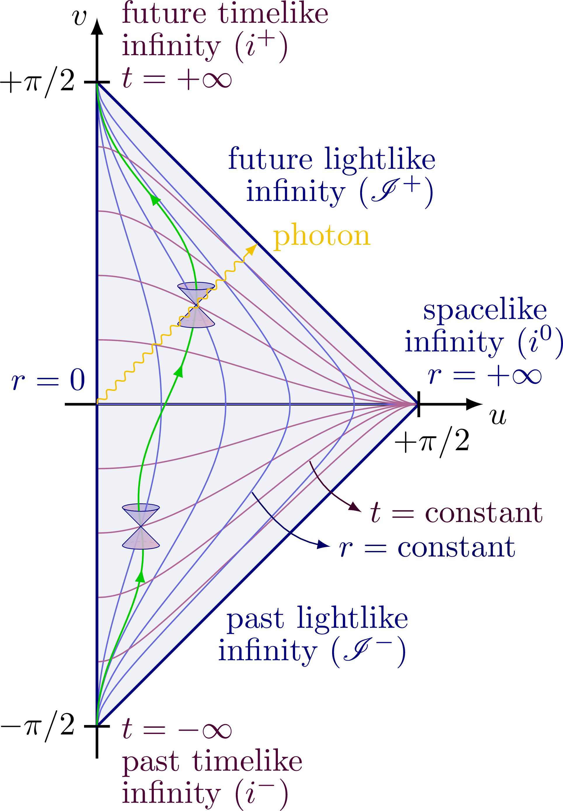
Penrose diagram of Minkowski and Schwarzschild metrics to illustrate the causal structure of different spacetime geometries. Lightlike worldlines remain at 45 degrees as indicated by the photons and light cones, i.e. the diagrams are conformal. The grid indicates lines of constant r and t. Different types of infinities are indicated: lightlike, timelike, spacelike, postive/negative future and past. For more related figures, please see Relativity category.
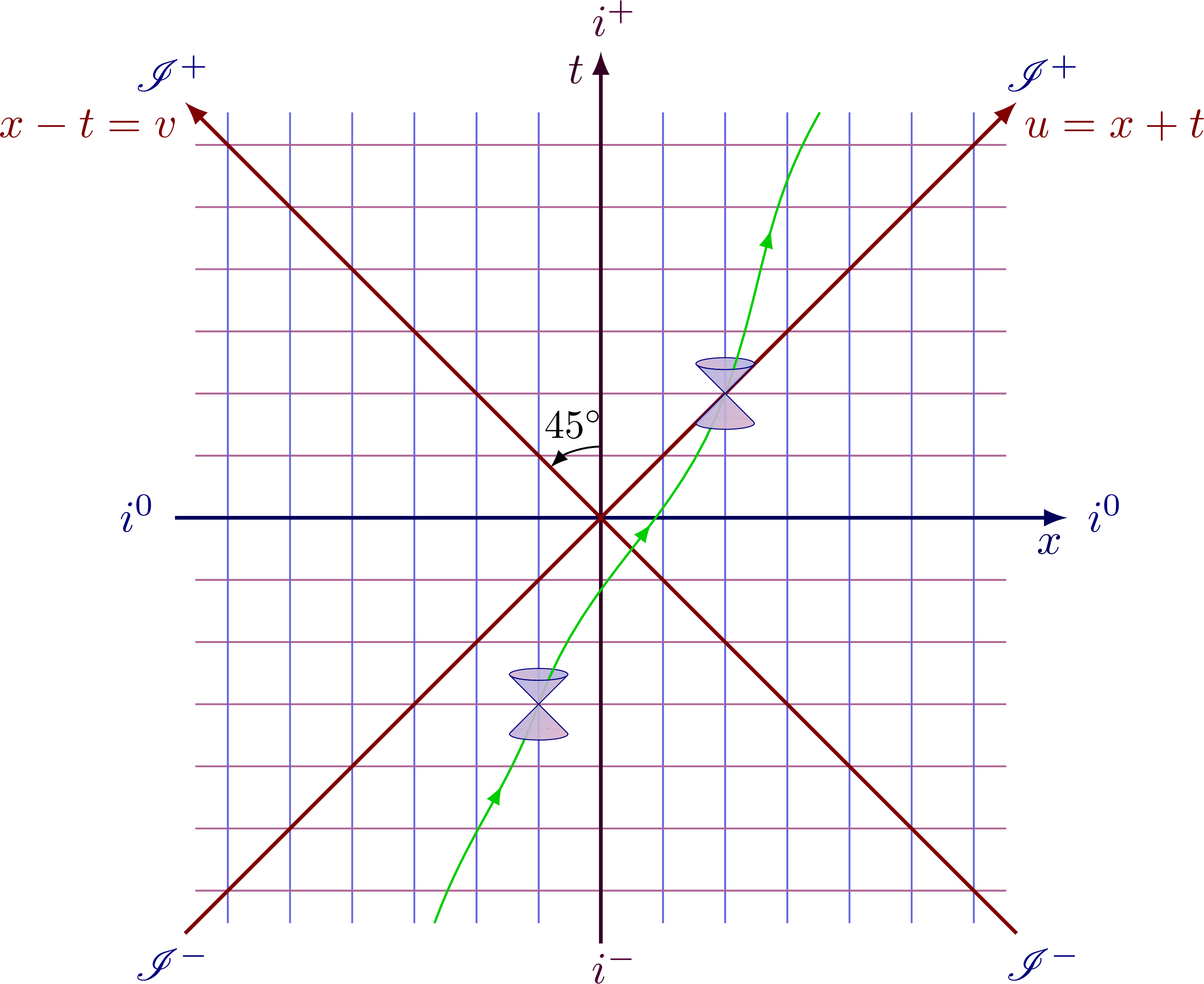
Simple coordinate transformation to rotate the axes by 45°.
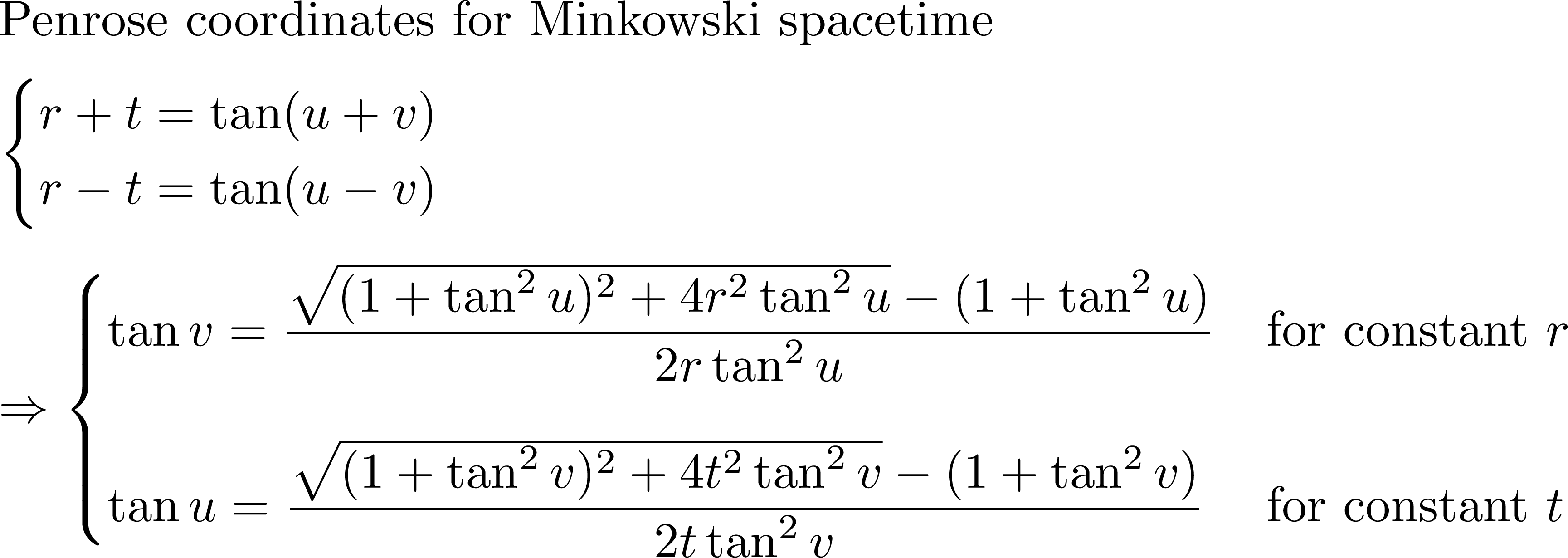
Transformation to Penrose coordinates for Minkowski space such that we can show infinity as a boundary:
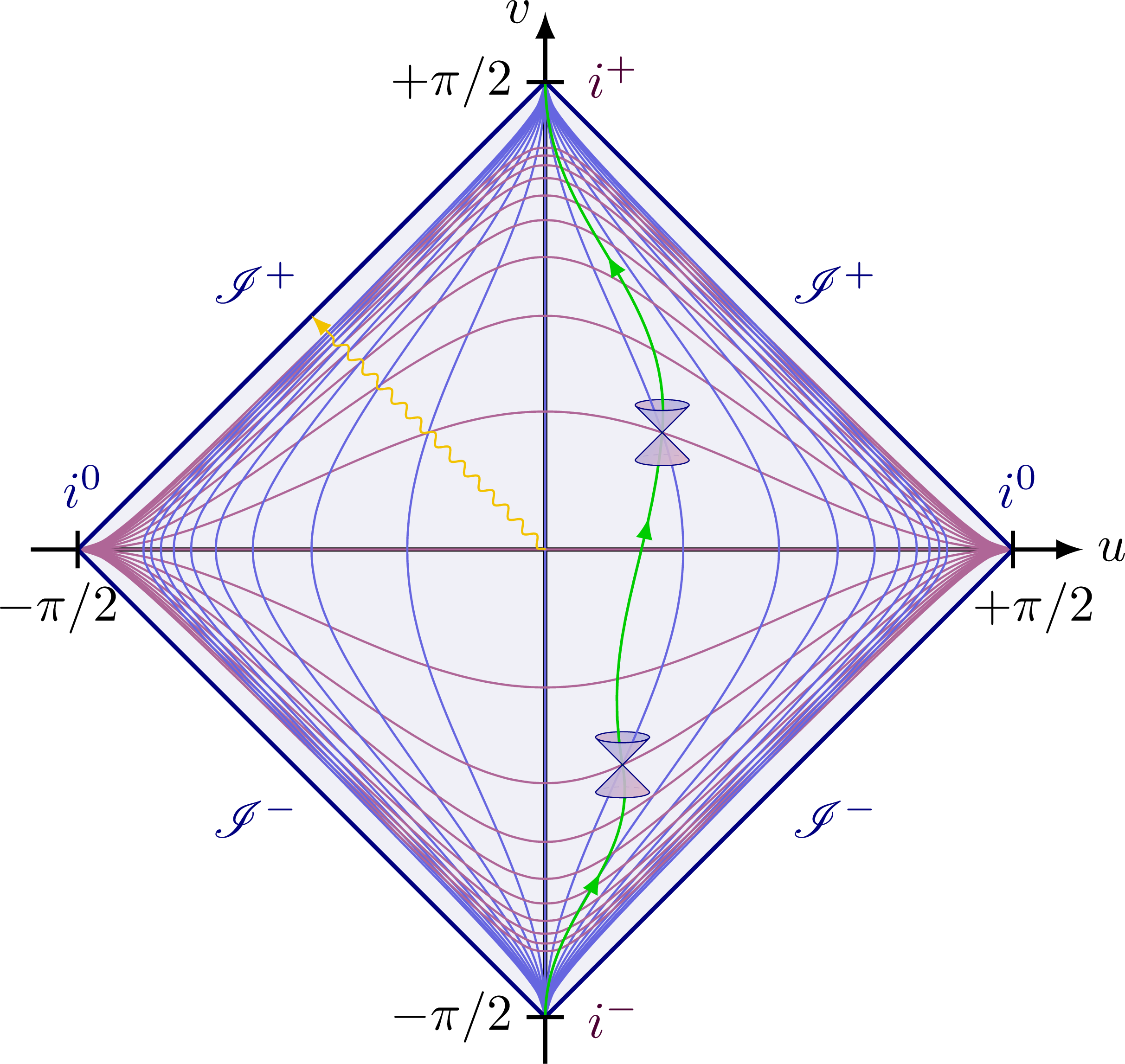
Penrose diagram with a particle worldliness and a light cone with 45° angles. The lines of constant time or constant space are equidistant in spacetime:
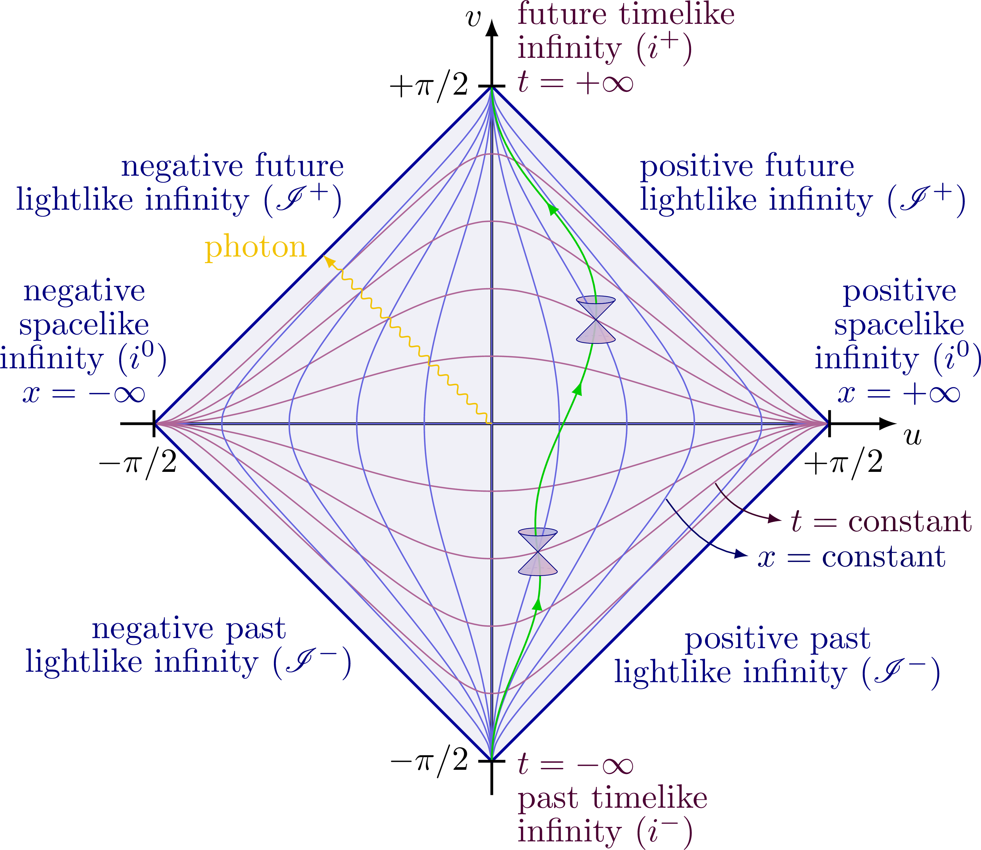
Penrose diagram with full labeling (note the lines of constant time or constant space are not equidistant in xt spacetime, but equidistant in uv spacetime instead):
Penrose diagram for radius r between 0 and infinity (instead of x):
Transformation of Kruskal-Szekeres coordinates to show the geometry of a Schwarzschild black hole:
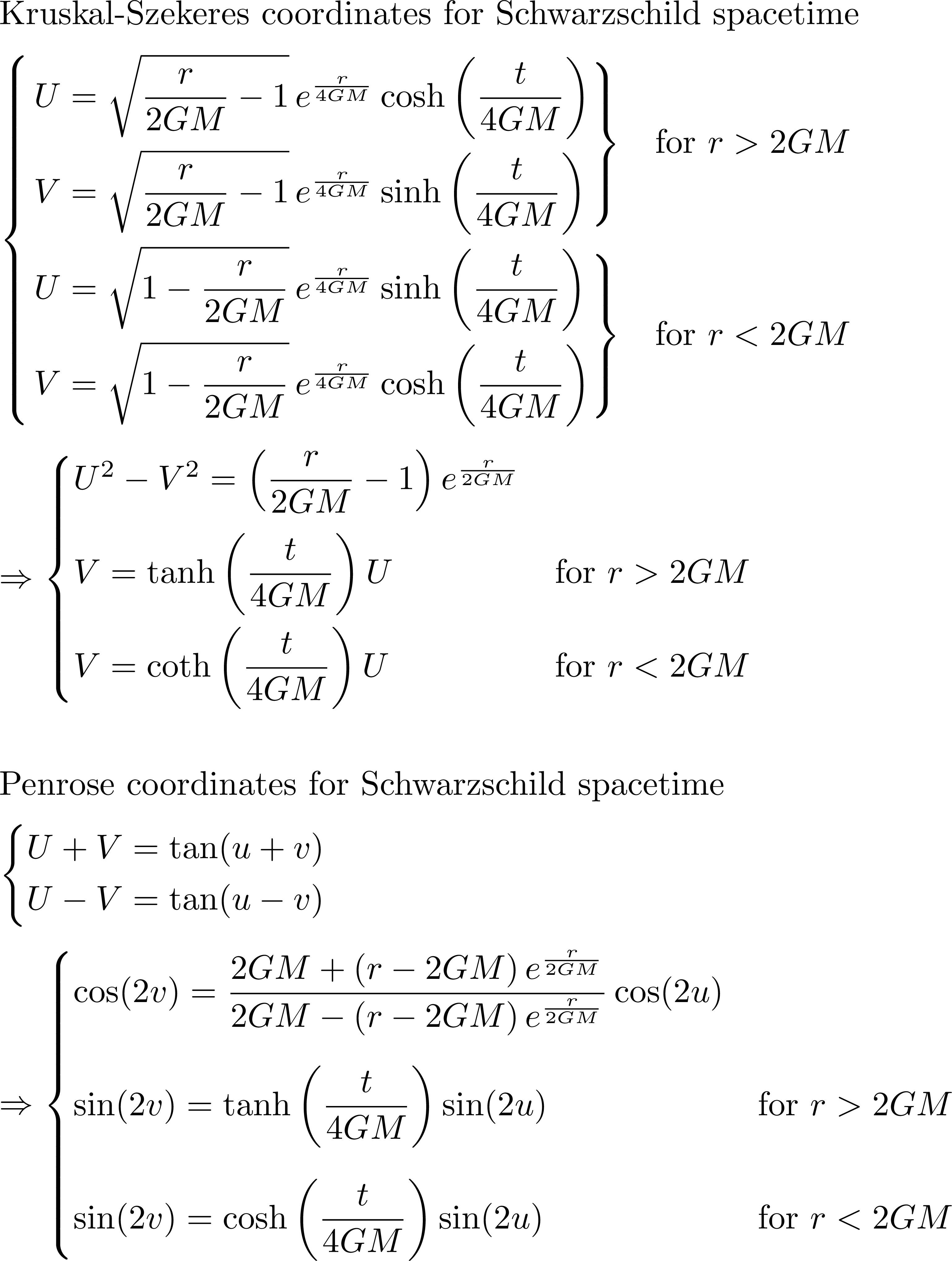
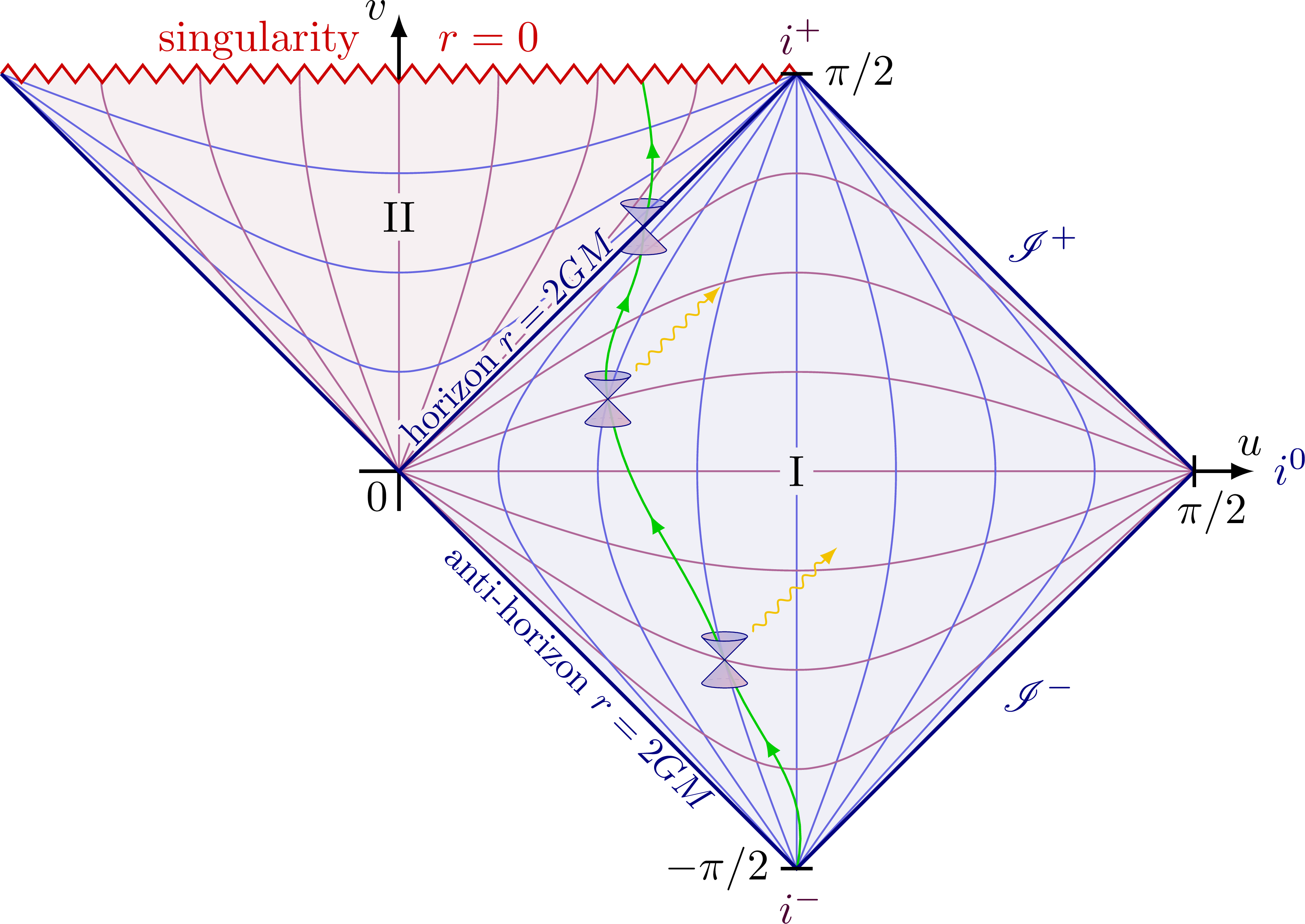
Penrose diagram for Schwarzschild black hole. It is derived via Kruskal-Szekeres coordinates above. The horizon is at r = 2GM (v = ±u), singularity at r = 0:
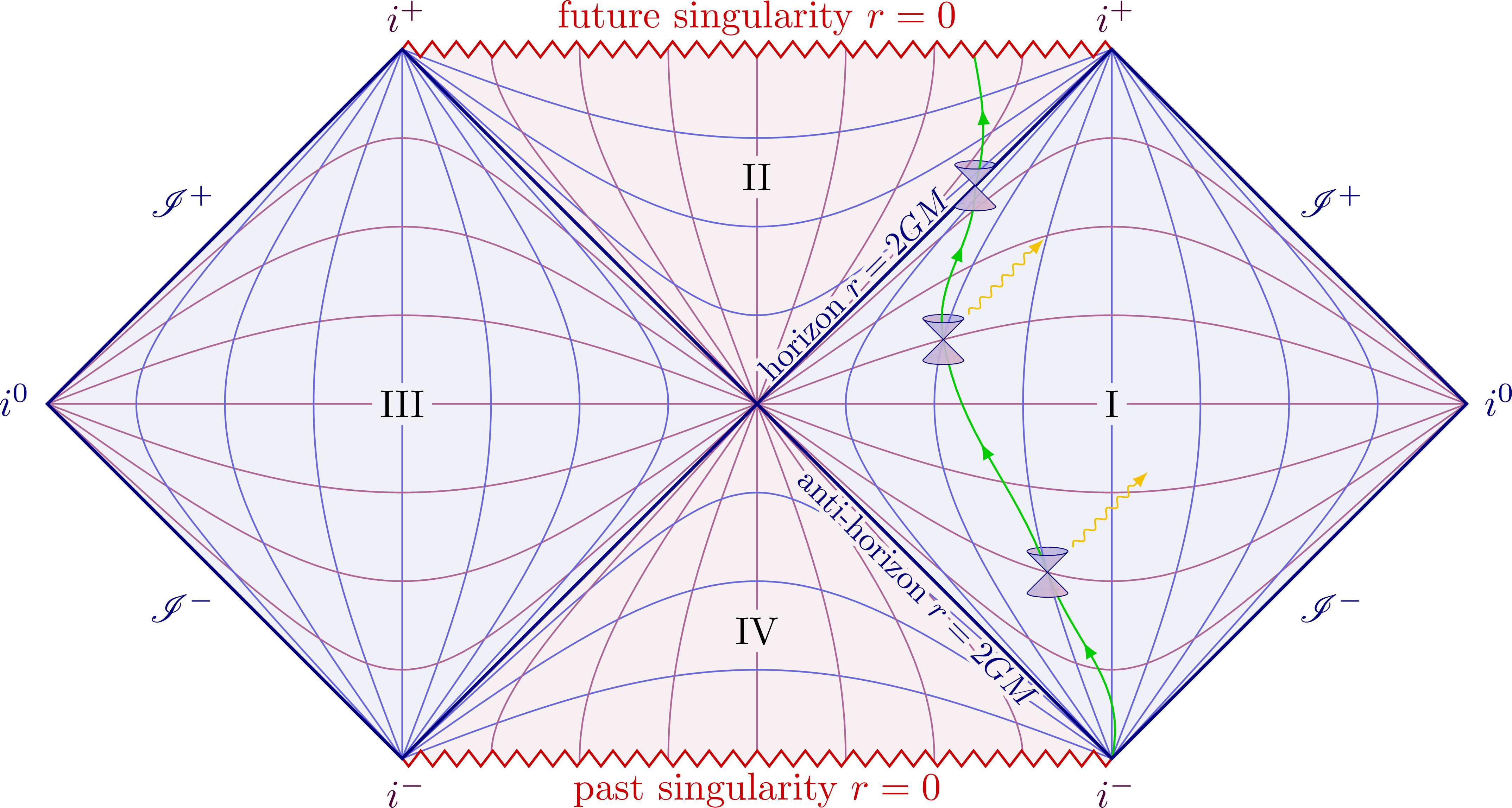
Extended Penrose diagram for Schwarzschild black hole:
Edit and compile if you like:
% Author: Izaak Neutelings (September 2021)
% Inspiration:
%   https://jila.colorado.edu/~ajsh/insidebh/penrose.html
%   https://tex.stackexchange.com/questions/99124/how-to-draw-penrose-diagrams-with-tikz
%   coordinates: https://arxiv.org/pdf/physics/0611033.pdf
%   https://arxiv.org/pdf/0711.0873.pdf
\documentclass[border=3pt,tikz]{standalone}
\usepackage{tikz}
\usepackage{amsmath} % for \text
\usepackage{mathrsfs} % for \mathscr
\usepackage{xfp} % higher precision (16 digits?)
\usepackage[outline]{contour} % glow around text
\usetikzlibrary{decorations.markings,decorations.pathmorphing}
\usetikzlibrary{angles,quotes} % for pic (angle labels)
\usetikzlibrary{arrows.meta} % for arrow size
\contourlength{1.4pt}

\newcommand{\calI}{\mathscr{I}} %\mathcal
\tikzset{>=latex} % for LaTeX arrow head
\colorlet{myred}{red!80!black}
\colorlet{myblue}{blue!80!black}
\colorlet{mygreen}{green!80!black}
\colorlet{mydarkred}{red!50!black}
\colorlet{mydarkblue}{blue!50!black}
\colorlet{mylightblue}{mydarkblue!6}
\colorlet{mypurple}{blue!40!red!80!black}
\colorlet{mydarkpurple}{blue!40!red!50!black}
\colorlet{mylightpurple}{mydarkpurple!80!red!6}
\colorlet{myorange}{orange!40!yellow!95!black}
\tikzstyle{cone}=[mydarkblue,line width=0.2,top color=blue!60!black!30,
                  bottom color=blue!60!black!50!red!30,shading angle=60,fill opacity=0.9]
\tikzstyle{cone back}=[mydarkblue,line width=0.1,dash pattern=on 1pt off 1pt]
\tikzstyle{world line}=[myblue!60,line width=0.4]
\tikzstyle{world line t}=[mypurple!60,line width=0.4]
\tikzstyle{particle}=[mygreen,line width=0.5]
\tikzstyle{photon}=[-{Latex[length=4,width=3]},myorange,line width=0.4,decorate,
                    decoration={snake,amplitude=0.9,segment length=4,post length=3.8}]
\tikzstyle{singularity}=[myred,line width=0.6,decorate,
                         decoration={zigzag,amplitude=2,segment length=6.17}]
\tikzset{declare function={%
  penrose(\x,\c)  = {\fpeval{2/pi*atan( (sqrt((1+tan(\x)^2)^2+4*\c*\c*tan(\x)^2)-1-tan(\x)^2) /(2*\c*tan(\x)^2) )}};%
  penroseu(\x,\t) = {\fpeval{atan(\x+\t)/pi+atan(\x-\t)/pi}};%
  penrosev(\x,\t) = {\fpeval{atan(\x+\t)/pi-atan(\x-\t)/pi}};%
  kruskal(\x,\c)  = {\fpeval{asin( \c*sin(2*\x) )*2/pi}};% Penrose coordinates for Kruskal
}}
\def\tick#1#2{\draw[thick] (#1) ++ (#2:0.04) --++ (#2-180:0.08)}
\def\Nsamples{20} % number samples in plot

% LIGHTCONE
\def\R{0.08} % size lightcone
\def\e{0.08} % vertical scale
\def\ang{45} % angle light cone
\def\angb{acos(sqrt(\e)*sin(\ang))} % angle ellipse center to point of tangency
\def\a{\R*sin(\ang)*sqrt(1-\e*sin(\ang)^2)/(1-\e*sin(\ang)^2)} % vertical radius
\def\b{\R*sqrt(\e)*sin(\ang)*cos(\ang)/(1-\e*sin(\ang)^2)} % horizontal radius
\def\coneback#1{ % light cone part to be drawn behind world lines
  \draw[cone back] % dashed line back
    (#1)++(-45:\R) arc({90-\angb}:{90+\angb}:{\a} and {\b});
  \draw[cone,shading angle=-60] % top edge & inside
    (#1)++(0,{\R*cos(\ang)/(1-\e*sin(\ang)^2)}) ellipse({\a} and {\b});
}
\def\conefront#1{ % light cone part to be drawn over world lines
  \draw[cone] % light cone outside
    (#1) --++ (45:\R) arc({\angb-90}:{-90-\angb}:{\a} and {\b})
     --++ (-45:2*\R) arc({90-\angb}:{-270+\angb}:{\a} and {\b}) -- cycle;
}

\begin{document}


% PENROSE DIAGRAM of Minkowski space - 45 rotation
\begin{tikzpicture}[scale=3.2]
  \message{Penrose diagram (45 rotation)^^J}

  \def\R{0.10} % size lightcone
  \def\Nlines{6} % number of world lines (at constant r/t)
  \pgfmathsetmacro\d{0.92/\Nlines} % grid size

  \coordinate (O) at (0,0);
  \coordinate (W) at (-1.05,0);
  \coordinate (E) at (1.15,0);
  \coordinate (S) at (0,-1.05);
  \coordinate (N) at (0,1.15);
  \coordinate (SW) at (-135:1.45);
  \coordinate (SE) at (-45:1.45);
  \coordinate (NW) at (135:1.45);
  \coordinate (NE) at (45:1.45);
  \coordinate (X0) at (-0.41,-1);
  \coordinate (X1) at (-\d,-3*\d);
  \coordinate (X2) at (2*\d,2*\d);
  \coordinate (X3) at (0.54,1);

  % WORLD LINES GRID
  \message{Making world lines...^^J}
  \foreach \i [evaluate={\x=\i*\d;}] in {1,...,\Nlines}{
    \message{  Running i/N=\i/\Nlines, x=\x...^^J}
    \draw[world line]   (-\x,-1) -- (-\x,1);
    \draw[world line]   ( \x,-1) -- ( \x,1);
    \draw[world line t] (-1,-\x) -- (1,-\x);
    \draw[world line t] (-1, \x) -- (1, \x);
  }

  % AXES
  \draw[->,thick,mydarkblue!70!black]
    (W) -- (E) node[left=4,below=0] {$x$};
  \draw[->,thick,mydarkpurple!70!black]
    (S) -- (N) coordinate (N) node[below=4,left=0] {$t$};
  \draw[->,thick,mydarkred] (SW) -- (NE) node[below right=-2] {$u=x+t$};
  \draw[->,thick,mydarkred] (SE) -- (NW) node[below left=-2] {$x-t=v$};

  \draw pic[->,"$45^\circ$"{above,scale=0.9},draw=black,angle radius=16,
            angle eccentricity=1.0] {angle = N--O--NW};

  % INFINITY LABELS
  \node[above=1,left=1,mydarkblue] at (W) {$i^0$};
  \node[above=1,right=1,mydarkblue] at (E) {$i^0$};
  \node[right=3,below=2,mydarkpurple] at (0,-1) {$i^-$};
  \node[right=3,above=0,mydarkpurple] at (N) {$i^+$};
  \node[mydarkblue,left=5,below right=-1] at (SE) {$\calI^-$};
  \node[mydarkblue,right=8,below left=-1] at (SW) {$\calI^-$};
  \node[mydarkblue,left=5,above right=-1] at (NE) {$\calI^+$};
  \node[mydarkblue,right=8,above left=-1] at (NW) {$\calI^+$};

  % LIGHT CONE BACK
  \coneback{X1};
  \coneback{X2};

  % PARTICLE
  \draw[particle,decoration={markings,mark=at position 0.170 with {\arrow{latex}},
                                      mark=at position 0.505 with {\arrow{latex}},
                                      mark=at position 0.860 with {\arrow{latex}}},postaction={decorate}]
    (X0) to[out=70,in=-110] (X1) to[out=70,in=-110] (X2) to[out=70,in=-120] (X3);

  % LIGHT CONE FRONT
  \conefront{X1};
  \conefront{X2};

\end{tikzpicture}


% PENROSE COORDINATES for Minkowski spacetime
\begin{tikzpicture}[scale=1]
  \def\tu{\tan^2u} % shorthand
  \def\tv{\tan^2v} % shorthand
  \node[align=left] at (0,0)
    {Penrose coordinates for Minkowski spacetime\\[2mm]$
    \left\{\begin{aligned}
      r + t = \tan(u+v) \\
      r - t = \tan(u-v) \\
    \end{aligned}\right.$\\[2mm]$
    \Rightarrow\begin{cases}
      \tan v = \dfrac{\sqrt{(1+\tu)^2+4r^2\tu}-(1+\tu)}{2r\tu} & \text{for constant $r$} \\[5mm]
      \tan u = \dfrac{\sqrt{(1+\tv)^2+4t^2\tv}-(1+\tv)}{2t\tv} & \text{for constant $t$}
    \end{cases}$};
\end{tikzpicture}


% PENROSE DIAGRAM of Minkowski space - equidistant world lines
\begin{tikzpicture}[scale=3.2]
  \message{Penrose diagram (equidistant world lines)^^J}

  \def\Nlines{9} % number of world lines (at constant r/t)
  \def\d{0.5}
  \coordinate (O) at ( 0, 0); % center: origin (r,t) = (0,0)
  \coordinate (S) at ( 0,-1); % south: t=-infty, i-
  \coordinate (N) at ( 0, 1); % north: t=+infty, i+
  \coordinate (W) at (-1, 0); % east:  r=-infty, i0
  \coordinate (E) at ( 1, 0); % west:  r=+infty, i0
  \coordinate (X) at ({penroseu(\d,\d)},{penrosev(\d,\d)});
  \coordinate (X0) at ({penroseu(\d,-2*\d)},{penrosev(\d,-2*\d)});

  % AXES
  \fill[mylightblue] (N) -- (E) -- (S) -- (W) -- cycle;
  \draw[->,thick] (-1.1,0) -- (1.15,0) node[right=-1] {$u$};
  \draw[->,thick] (0,-1.1) -- (0,1.15) node[left=-1] {$v$};

  % INFINITY LABELS
  \node[right=1,above=1,mydarkblue] at (-1,0.04) {$i^0$};
  \node[right=1,above=1,mydarkblue] at (1,0.04) {$i^0$};
  \node[below=0,right=1,mydarkpurple] at (0.04,-1) {$i^-$};
  \node[above=1,right=1,mydarkpurple] at (0.04,1) {$i^+$};
  \node[mydarkblue,below left=-1] at (-0.5,-0.5) {$\calI^-$};
  \node[mydarkblue,above left=-1] at (-0.5,0.5) {$\calI^+$};
  \node[mydarkblue,above right=-1] at (0.5,0.5) {$\calI^+$};
  \node[mydarkblue,below right=-1] at (0.5,-0.5) {$\calI^-$};

  % LIGHT CONE BACK
  \coneback{X};
  \coneback{X0};

  % WORLD LINES
  \draw[world line] (N) -- (S);
  \draw[world line t] (W) -- (E);
  \message{Making world lines...^^J}
  \foreach \i [evaluate={\c=\i*\d;}] in {1,...,\Nlines}{
    \message{  Running i/N=\i/\Nlines, c=\c...^^J}
    \draw[world line t,samples=\Nsamples,smooth,variable=\x,domain=-1:1] % constant t
      plot(\x,{-penrose(\x*pi/2,\c)})
      plot(\x,{ penrose(\x*pi/2,\c)});
    \draw[world line,samples=\Nsamples,smooth,variable=\y,domain=-1:1] % constant r
      plot({-penrose(\y*pi/2,\c)},\y)
      plot({ penrose(\y*pi/2,\c)},\y);
  }
  \draw[thick,mydarkblue] (N) -- (E) -- (S) -- (W) -- cycle;

  % PARTICLE
  \draw[particle,decoration={markings,mark=at position 0.16 with {\arrow{latex}},
                                      mark=at position 0.53 with {\arrow{latex}},
                                      mark=at position 0.81 with {\arrow{latex}}},postaction={decorate}]
    (S) to[out=90,in=-80] (X0) to[out=100,in=-95] (X) to[out=85,in=-90] (N);

  % LIGHT CONE FRONT
  \conefront{X};
  \conefront{X0};

  % PHOTON
  \draw[->,photon] (O) -- (-0.5,0.5); %node[above=2,right=1] {photon};

  % TICKS
  \tick{W}{90} node[left=4,below=-1] {$-\pi/2$};
  \tick{E}{90} node[right=4,below=-1] {$+\pi/2$};
  \tick{S}{ 0} node[left=-1] {$-\pi/2$};
  \tick{N}{ 0} node[left=-1] {$+\pi/2$};

\end{tikzpicture}


% PENROSE DIAGRAM of Minkowski space
\begin{tikzpicture}[scale=3.5]
  \message{Penrose diagram^^J}

  \def\Nlines{4} % number of world lines (at constant r/t)
  \def\ta{tan(90*1.0/(\Nlines+1))} % constant r/t value 1
  \def\tb{tan(90*2.0/(\Nlines+1))} % constant r/t value 2
  \coordinate (O) at ( 0, 0); % center: origin (r,t) = (0,0)
  \coordinate (S) at ( 0,-1); % south: t=-infty, i-
  \coordinate (N) at ( 0, 1); % north: t=+infty, i+
  \coordinate (W) at (-1, 0); % east:  r=-infty, i0
  \coordinate (E) at ( 1, 0); % west:  r=+infty, i0
  \coordinate (X) at ({penroseu(\tb,\tb)},{penrosev(\tb,\tb)});
  \coordinate (X0) at ({penroseu(\ta,-\tb)},{penrosev(\ta,-\tb)});

  % AXES
  \fill[mylightblue] (N) -- (E) -- (S) -- (W) -- cycle;
  \draw[->,thick] (-1.1,0) -- (1.2,0) node[below right=-2] {$u$};
  \draw[->,thick] (0,-1.1) -- (0,1.2) node[left=-1] {$v$};

  % INFINITY LABELS
  \node[right=6,above left=-2,mydarkblue,align=center] at (-1,0.04)
    {negative\\[-2]spacelike\\[-2]infinity ($i^0$)\\[-2]$x=-\infty$};
  \node[left=6,above right=-2,mydarkblue,align=center] at (1,0.04)
    {positive\\[-2]spacelike\\[-2]infinity ($i^0$)\\[-2]$x=+\infty$};
  \node[above=6,below right=0,mydarkpurple,align=left] at (0.04,-1)
    {$t=-\infty$\\[-2]past timelike\\[-2]infinity ($i^-$)};
  \node[below=6,above right=0,mydarkpurple,align=left] at (0.04,1)
    {future timelike\\[-2]infinity ($i^+$)\\[-2]$t=+\infty$};
  \node[mydarkblue,above right,align=left] at (55:0.7)
    {positive future\\[-2]lightlike infinity ($\calI^+$)};
  \node[mydarkblue,below right,align=center] at (-60:0.65)
    {positive past\\[-2]lightlike infinity ($\calI^-$)};
  \node[mydarkblue,above left,align=right] at (125:0.7)
    {negative future\\[-2]lightlike infinity ($\calI^+$)};
  \node[mydarkblue,below left,align=center] at (-125:0.65)
    {negative past\\[-2]lightlike infinity ($\calI^-$)};

  % CONE BACK
  \coneback{X};
  \coneback{X0};

  % WORLD LINES
  \draw[world line] (N) -- (S);
  \draw[world line] (W) -- (E);
  \message{Making world lines...^^J}
  \foreach \i [evaluate={\c=\i/(\Nlines+1); \ct=tan(90*\c);}] in {1,...,\Nlines}{
    \message{  Running i/N=\i/\Nlines, c=\c, tan(90*\c)=\ct...^^J}
    \draw[world line t,samples=\Nsamples,smooth,variable=\t,domain=-1:1] % constant t
      plot(\t,{-penrose(\t*pi/2,\ct)})
      plot(\t,{ penrose(\t*pi/2,\ct)});
    \draw[world line,samples=\Nsamples,smooth,variable=\x,domain=-1:1] % constant r
      plot({-penrose(\x*pi/2,\ct)},\x)
      plot({ penrose(\x*pi/2,\ct)},\x);
  }
  \draw[thick,blue!60!black] (N) -- (E) -- (S) -- (W) -- cycle;

  % CONSTANT
  \draw[->,mydarkpurple!80!black,shorten <=0.4] % constant r
    (0.66,{-penrose(0.66*pi/2,tan(90*3/(\Nlines+1)))}) to[out=-60,in=170]++ (-30:0.23)
    node[right=-1] {$t=\text{constant}$};
  \draw[->,mydarkblue!80!black,shorten <=0.4] % constant t
    ({penrose(-0.22*pi/2,tan(90*3/(\Nlines+1)))},-0.22) to[out=-55,in=170]++ (-35:0.3)
    node[right=-1] {$x=\text{constant}$};

  % PARTICLE
  \draw[particle,decoration={markings,mark=at position 0.24 with {\arrow{latex}},
                                      mark=at position 0.55 with {\arrow{latex}},
                                      mark=at position 0.82 with {\arrow{latex}}},postaction={decorate}]
    (S) to[out=90,in=-80] (X0) to[out=100,in=-95] (X) to[out=85,in=-90] (N);

  % LIGHT CONE FRONT
  \conefront{X};
  \conefront{X0};

  % PHOTON
  \draw[->,photon] (O) -- (-0.5,0.5) node[above=2,left=1] {photon};

  % TICKS
  \tick{W}{90} node[left=5,below=-1] {$-\pi/2$};
  \tick{E}{90} node[right=4,below=-1] {$+\pi/2$};
  \tick{S}{ 0} node[left=-1] {$-\pi/2$};
  \tick{N}{ 0} node[left=-1] {$+\pi/2$};

\end{tikzpicture}


% PENROSE DIAGRAM of Minkowski space - radius r
\begin{tikzpicture}[scale=3.5]
  \message{Penrose diagram (radius r)^^J}

  \def\Nlines{4} % number of world lines (at constant r/t)
  \def\ta{tan(90*1.0/(\Nlines+1))} % constant r/t value 1
  \def\tb{tan(90*2.0/(\Nlines+1))} % constant r/t value 2
  \coordinate (O) at ( 0, 0); % center: origin (r,t) = (0,0)
  \coordinate (S) at ( 0,-1); % south: t=-infty, i-
  \coordinate (N) at ( 0, 1); % north: t=+infty, i+
  \coordinate (E) at ( 1, 0); % east:  r=+infty, i0
  \coordinate (X) at ({penroseu(\tb,\tb)},{penrosev(\tb,\tb)});
  \coordinate (X0) at ({penroseu(\ta,-\tb)},{penrosev(\ta,-\tb)});

  % AXES
  \fill[mylightblue] (N) -- (E) -- (S) -- cycle;
  \draw[->,thick] (-0.1,0) -- (1.2,0) node[below right=-2] {$u$};
  \draw[->,thick] (0,-1.1) -- (0,1.2) node[left=-1] {$v$};

  % INFINITY LABELS
  \node[above=1,above left=0,mydarkblue,align=center] at (O)
    {$r=0$};
  \node[left=6,above right=-2,mydarkblue,align=center] at (1,0.04)
    {spacelike\\[-2]infinity ($i^0$)\\[-2]$r=+\infty$};
  \node[above=6,below right=0,mydarkpurple,align=left] at (0.04,-1)
    {$t=-\infty$\\[-2]past timelike\\[-2]infinity ($i^-$)};
  \node[below=6,above right=0,mydarkpurple,align=left] at (0.04,1)
    {future timelike\\[-2]infinity ($i^+$)\\[-2]$t=+\infty$};
  \node[mydarkblue,above right,align=right] at (57:0.68)
    {future lightlike\\[-2]infinity ($\calI^+$)};
  \node[mydarkblue,below right,align=right] at (-60:0.68)
    {past lightlike\\[-2]infinity ($\calI^-$)};

  % CONE BACK
  \coneback{X};
  \coneback{X0};

  % WORLD LINES
  \draw[world line] (N) -- (S);
  \draw[world line] (O) -- (E);
  \message{Making world lines...^^J}
  \foreach \i [evaluate={\c=\i/(\Nlines+1); \ct=tan(90*\c);}] in {1,...,\Nlines}{
    \message{  Running i/N=\i/\Nlines, c=\c, tan(90*\c)=\ct...^^J}
    \draw[world line t,samples=\Nsamples,smooth,variable=\t,domain=0.001:1] % constant t
      plot(\t,{-penrose(\t*pi/2,\ct)})
      plot(\t,{ penrose(\t*pi/2,\ct)});
    \draw[world line,samples=\Nsamples,smooth,variable=\r,domain=-1:1] % constant r
      plot({penrose(\r*pi/2,\ct)},\r);
  }
  \draw[thick,mydarkblue] (N) -- (E) -- (S) -- cycle;

  % CONSTANT
  \draw[->,mydarkpurple!80!black,shorten <=0.4] % constant r
    (0.66,{-penrose(0.66*pi/2,tan(90*3/(\Nlines+1)))}) to[out=-70,in=150]++ (-45:0.23)
    node[right=-1] {$t=\text{constant}$};
  \draw[->,mydarkblue!80!black,shorten <=0.4] % constant t
    ({penrose(-0.27*pi/2,tan(90*3/(\Nlines+1)))},-0.27) to[out=-55,in=170]++ (-35:0.3)
    node[right=-1] {$r=\text{constant}$};

  % PARTICLE
  \draw[particle,decoration={markings,mark=at position 0.24 with {\arrow{latex}},
                                      mark=at position 0.55 with {\arrow{latex}},
                                      mark=at position 0.82 with {\arrow{latex}}},postaction={decorate}]
    (S) to[out=90,in=-80] (X0) to[out=100,in=-95] (X) to[out=85,in=-90] (N);

  % LIGHT CONE FRONT
  \conefront{X};
  \conefront{X0};

  % PHOTON
  \draw[->,photon] (O) -- (0.5,0.5) node[above=2,right=1] {photon};

  % TICKS
  \tick{E}{90} node[right=4,below=-1] {$+\pi/2$};
  \tick{S}{ 0} node[left=-1] {$-\pi/2$};
  \tick{N}{ 0} node[left=-1] {$+\pi/2$};

\end{tikzpicture}


% PENROSE COORDINATES for Kruskal-Szekeres coordinates
\begin{tikzpicture}[scale=1]
  \def\tu{\tan^2u} % shorthand
  \def\tv{\tan^2v} % shorthand
  \node[align=left] at (0,0) {
    Kruskal-Szekeres coordinates for Schwarzschild spacetime\\[2mm]
    $\displaystyle
    \begin{cases}
      \left.\begin{aligned}
        U &= \sqrt{\frac{r}{2GM}-1}\,e^{\frac{r}{4GM}}\cosh\left(\frac{t}{4GM}\right) \\
        V &= \sqrt{\frac{r}{2GM}-1}\,e^{\frac{r}{4GM}}\sinh\left(\frac{t}{4GM}\right) \\
      \end{aligned}\right\} &\text{for $r>2GM$} \\[8mm]
      \left.\begin{aligned}
        U &= \sqrt{1-\frac{r}{2GM}}\,e^{\frac{r}{4GM}}\sinh\left(\frac{t}{4GM}\right) \\
        V &= \sqrt{1-\frac{r}{2GM}}\,e^{\frac{r}{4GM}}\cosh\left(\frac{t}{4GM}\right) \\
      \end{aligned}\right\} &\text{for $r<2GM$}
    \end{cases}$\\[2mm]
    $\displaystyle
    \Rightarrow\begin{cases}
      U^2 - V^2 = \left(\dfrac{r}{2GM}-1\right)e^{\frac{r}{2GM}} \\[3mm]
      V = \tanh\left(\dfrac{t}{4GM}\right)U & \text{for $r>2GM$} \\[3mm]
      V = \coth\left(\dfrac{t}{4GM}\right)U & \text{for $r<2GM$}
    \end{cases}$\\[6mm]
    Penrose coordinates for Schwarzschild spacetime\\[2mm]$
    \left\{\begin{aligned}
      U + V = \tan(u+v) \\
      U - V = \tan(u-v) \\
    \end{aligned}\right.$\\[2mm]
    $\displaystyle
    \Rightarrow\begin{cases}
      \cos(2v) = \dfrac{2GM+\left(r-2GM\right)e^{\frac{r}{2GM}}}
                       {2GM-\left(r-2GM\right)e^{\frac{r}{2GM}}}
                 \cos(2u) \\[5mm]
      \sin(2v) = \tanh\left(\dfrac{t}{4GM}\right)\sin(2u) & \text{for $r>2GM$} \\[5mm]
      \sin(2v) = \cosh\left(\dfrac{t}{4GM}\right)\sin(2u) & \text{for $r<2GM$}
    \end{cases}$};
\end{tikzpicture}


% PENROSE DIAGRAM of a Schwarzschild black hole
\begin{tikzpicture}[scale=3.2]
  \message{Extended Penrose diagram: Schwarzschild black hole^^J}

  \def\R{0.08} % size lightcone
  \def\Nlines{3} % number of world lines (at constant r/t)
  \pgfmathsetmacro\ta{1/sin(90*1/(\Nlines+1))} % constant r/t value 1
  \pgfmathsetmacro\tb{sin(90*2/(\Nlines+1))}   % constant r/t value 2
  \pgfmathsetmacro\tc{1/sin(90*2/(\Nlines+1))} % constant r/t value 3
  \pgfmathsetmacro\td{sin(90*1/(\Nlines+1))}   % constant r/t value 4
  \coordinate (-O) at (-1, 0); % center III: origin (r,t) = (0,0)
  \coordinate (-N) at (-1, 1); % north III: t=+infty, i+
  \coordinate (O)  at ( 1, 0); % center I: origin (r,t) = (0,0)
  \coordinate (S)  at ( 1,-1); % south I: t=-infty, i-
  \coordinate (N)  at ( 1, 1); % north I: t=+infty, i+
  \coordinate (E)  at ( 2, 0); % east I:  r=-infty, i0
  \coordinate (W)  at ( 0, 0); % west I:  r=+infty, i0
  \coordinate (B)  at ( 0,-1); % singularity bottom
  \coordinate (X0) at ({asin(sqrt((\ta^2-1)/(\ta^2-\tb^2)))/90},
                       {-acos(\ta*sqrt((1-\tb^2)/(\ta^2-\tb^2)))/90}); % particle 1
  \coordinate (X1) at ({asin(sqrt((\tc^2-1)/(\tc^2-\td^2)))/90},
                       {acos(\tc*sqrt((1-\td^2)/(\tc^2-\td^2)))/90}); % particle 2
  \coordinate (X2) at (45:0.87); % particle falling in BH horizon
  \coordinate (X3) at (0.60,1.05); % particle falling in BH singularity

  % AXES
  \draw[->,thick] (0,-0.1) -- (0,1.15) node[above=1,left=-1] {$v$};
  \draw[->,thick] (-0.1,0) -- (2.15,0) node[left=1,above=0] {$u$};

  \begin{scope}

    % CLIP to fill inside zigzag lines
    \clip[decorate,decoration={zigzag,amplitude=2,segment length=6.17}]
      (-N) -- (N) --++ (1.1,0.1) |-++ (-3.1,-2.3) -- cycle;

    % REGIONS FILLS
    \fill[mylightpurple] (-N) |-++ (2,0.1) -- (N) -- (W) -- cycle;
    \fill[mylightblue] (N) -- (E) -- (S) -- (W) -- cycle;

    % CONE BACK
    \coneback{X0};
    \coneback{X1};
    \coneback{X2};

    % WORLD LINES
    \draw[world line] (N) -- (S);
    \draw[world line t] (W) -- (E) (W) -- (0,1.1);
    \message{Making world lines...^^J}
    \foreach \i [evaluate={\c=\i/(\Nlines+1); \cs=sin(90*\c);}] in {1,...,\Nlines}{
      \message{  Running i/N=\i/\Nlines, c=\c, cs=\cs...^^J}
      \draw[world line t,samples=\Nsamples,smooth,variable=\x,domain=0:2] % region I, constant t
        plot(\x,{-kruskal(\x*pi/4,\cs)})
        plot(\x,{ kruskal(\x*pi/4,\cs)});
      \draw[world line,samples=\Nsamples,smooth,variable=\y,domain=0:2] % region I, constant r
        plot({1-kruskal(\y*pi/4,\cs)},\y-1)
        plot({1+kruskal(\y*pi/4,\cs)},\y-1);
      \draw[world line,samples=\Nsamples,smooth,variable=\x,domain=0:2] % region II, constant r
        plot(\x-1,{1-kruskal(\x*pi/4,\cs)});
      \draw[world line t,samples=\Nsamples,smooth,variable=\y,domain=0:1.05] % region II constant t
        plot({-kruskal(\y*pi/4,\cs)},\y)
        plot({ kruskal(\y*pi/4,\cs)},\y);
    }

    % PARTICLE WORLD LINE
    \draw[particle,decoration={markings,mark=at position 0.16 with {\arrow{latex}},
                                        mark=at position 0.45 with {\arrow{latex}},
                                        mark=at position 0.72 with {\arrow{latex}},
                                        mark=at position 0.90 with {\arrow{latex}}},postaction={decorate}]
      (S) to[out=77,in=-70] (X0) to[out=110,in=-80] (X1)
          to[out=100,in=-90] (X2) to[out=75,in=-80] (X3);

  \end{scope}

  % LIGHT CONE FRONT
  \conefront{X0};
  \conefront{X1};
  \conefront{X2};

  % ESCAPING PHOTONS
  \draw[photon] (X0) ++ (45:0.1) --++ (45:0.3);
  \draw[photon] (X1) ++ (45:0.1) --++ (45:0.3);

  % REGIONS
  \node[fill=mylightblue,inner sep=2] at (O) {I};
  \node[fill=mylightpurple,inner sep=2] at (0,0.64) {II};

  % BOUNDARIES
  \draw[singularity] (-N) -- node[pos=0.46,above left=-2] {\strut singularity} (N);
  \draw[singularity] (-N) -- node[pos=0.54,above right=-2] {\strut $r=0$} (N);
  \path (S) -- (W) node[mydarkblue,pos=0.50,below=-2.5,rotate=-45,scale=0.85]
    {anti-horizon $r=2GM$};
  \path (W) -- (N) node[mydarkblue,pos=0.32,above=-2.5,rotate=45,scale=0.85]
    {\contour{mylightpurple}{horizon $r=2GM$}};
  \draw[thick,mydarkblue] (N) -- (E) -- (S) --  (W) -- cycle;
  \draw[thick,mydarkblue] (W) -- (-N);

  % TICKS
  \node[below left=-1] at (W) {$0$};
  \tick{E}{90} node[right=4,below=-3] {$\pi/2$};
  \tick{S}{0} node[left=-1] {$-\pi/2$};
  \tick{N}{180} node[right=-1] {$\pi/2$};

  % INFINITY LABELS
  \node[above=1,right=1,mydarkblue] at (2.15,0) {$i^0$};
  \node[right=1,below=1,mydarkpurple] at (S) {$i^-$};
  \node[right=1,above=1,mydarkpurple] at (N) {$i^+$};
  \node[mydarkblue,above right=-1] at (1.5,0.5) {$\calI^+$};
  \node[mydarkblue,below right=-2] at (1.5,-0.5) {$\calI^-$};

\end{tikzpicture}


% EXTENDED PENROSE DIAGRAM of a Schwarzschild black hole
\begin{tikzpicture}[scale=3.2]
  \message{Extended Penrose diagram: Schwarzschild black hole^^J}

  \def\R{0.08} % size lightcone
  \def\Nlines{3} % number of world lines (at constant r/t)
  \pgfmathsetmacro\ta{1/sin(90*1/(\Nlines+1))} % constant r/t value 1
  \pgfmathsetmacro\tb{sin(90*2/(\Nlines+1))}   % constant r/t value 2
  \pgfmathsetmacro\tc{1/sin(90*2/(\Nlines+1))} % constant r/t value 3
  \pgfmathsetmacro\td{sin(90*1/(\Nlines+1))}   % constant r/t value 4
  \coordinate (-O) at (-1, 0); % center III: origin (r,t) = (0,0)
  \coordinate (-S) at (-1,-1); % south III: t=-infty, i-
  \coordinate (-N) at (-1, 1); % north III: t=+infty, i+
  \coordinate (-W) at (-2, 0); % east III:  r=-infty, i0
  \coordinate (-E) at ( 0, 0); % west III:  r=+infty, i0
  \coordinate (O)  at ( 1, 0); % center I: origin (r,t) = (0,0)
  \coordinate (S)  at ( 1,-1); % south I: t=-infty, i-
  \coordinate (N)  at ( 1, 1); % north I: t=+infty, i+
  \coordinate (E)  at ( 2, 0); % east I:  r=-infty, i0
  \coordinate (W)  at ( 0, 0); % west I:  r=+infty, i0
  \coordinate (B)  at ( 0,-1); % singularity bottom
  \coordinate (T)  at ( 0, 1); % singularity top
  \coordinate (X0) at ({asin(sqrt((\ta^2-1)/(\ta^2-\tb^2)))/90},
                       {-acos(\ta*sqrt((1-\tb^2)/(\ta^2-\tb^2)))/90}); % particle 1
  \coordinate (X1) at ({asin(sqrt((\tc^2-1)/(\tc^2-\td^2)))/90},
                       {acos(\tc*sqrt((1-\td^2)/(\tc^2-\td^2)))/90}); % particle 2
  \coordinate (X2) at (45:0.87); % particle falling in BH horizon
  \coordinate (X3) at (0.60,1.05); % particle falling in BH singularity

  \begin{scope}

    % CLIP to fill inside zigzag lines
    \clip[decorate,decoration={zigzag,amplitude=2,segment length=6.17}]
      (S) -- (-S) --++ (-1.1,-0.1) |-++ (4.2,2.2) |- cycle;
    \clip[decorate,decoration={zigzag,amplitude=2,segment length=6.17}]
      (-N) -- (N) --++ (1.1,0.1) |-++ (-4.2,-2.2) |- cycle;

    % REGIONS FILLS
    \fill[mylightpurple] (-N) |-++ (2,0.1) -- (N) -- (-S) -- (S) -- cycle;
    \fill[mylightpurple] (-S) |-++ (2,-0.1) -- (S) -- (-N) -- (N) -- cycle;

    \fill[mylightblue] (-N) -- (-E) -- (-S) -- (-W) -- cycle;
    \fill[mylightblue] (N) -- (E) -- (S) -- (W) -- cycle;

    % CONE BACK
    \coneback{X0};
    \coneback{X1};
    \coneback{X2};

    % WORLD LINES
    \draw[world line] (-N) -- (-S) (N) -- (S);
    \draw[world line t] (-W) -- (-E) (W) -- (E) (0,-1.1) -- (0,1.1);
    \message{Making world lines...^^J}
    \foreach \i [evaluate={\c=\i/(\Nlines+1); \cs=sin(90*\c);}] in {1,...,\Nlines}{
      \message{  Running i/N=\i/\Nlines, c=\c, cs=\cs...^^J}
      \draw[world line t,samples=2*\Nsamples,smooth,variable=\x,domain=-2:2] % region I/III, constant t
        plot(\x,{-kruskal(\x*pi/4,\cs)})
        plot(\x,{ kruskal(\x*pi/4,\cs)});
      \draw[world line,samples=\Nsamples,smooth,variable=\y,domain=0:2] % region I/III, constant r
        plot({-1-kruskal(\y*pi/4,\cs)},\y-1)
        plot({-1+kruskal(\y*pi/4,\cs)},\y-1)
        plot({1-kruskal(\y*pi/4,\cs)},\y-1)
        plot({1+kruskal(\y*pi/4,\cs)},\y-1);
      \draw[world line,samples=\Nsamples,smooth,variable=\x,domain=0:2] % region II/IV, constant r
        plot(\x-1,{kruskal(\x*pi/4,\cs)-1})
        plot(\x-1,{1-kruskal(\x*pi/4,\cs)});
      \draw[world line t,samples=\Nsamples,smooth,variable=\y,domain=-1.05:1.05] % region II/IV constant t
        plot({-kruskal(\y*pi/4,\cs)},\y)
        plot({ kruskal(\y*pi/4,\cs)},\y);
    }

    % PARTICLE WORLD LINE
    \draw[particle,decoration={markings,mark=at position 0.16 with {\arrow{latex}},
                                        mark=at position 0.45 with {\arrow{latex}},
                                        mark=at position 0.72 with {\arrow{latex}},
                                        mark=at position 0.90 with {\arrow{latex}}},postaction={decorate}]
      (S) to[out=77,in=-70] (X0) to[out=110,in=-80] (X1)
          to[out=100,in=-90] (X2) to[out=75,in=-80] (X3);

  \end{scope}

  % BOUNDARIES
  \draw[singularity] (-N) -- node[above] {future singularity $r=0$} (N);
  \draw[singularity] (S) -- node[below] {past singularity $r=0$} (-S);
  \path (S) -- (W) node[mydarkblue,pos=0.50,below=-2.5,rotate=-45,scale=0.85]
    {\contour{mylightpurple}{anti-horizon $r=2GM$}};
  \path (W) -- (N) node[mydarkblue,pos=0.32,above=-2.5,rotate=45,scale=0.85]
    {\contour{mylightpurple}{horizon $r=2GM$}};
  \draw[thick,mydarkblue] (-N) -- (-E) -- (-S) -- (-W) -- cycle;
  \draw[thick,mydarkblue] (N) -- (E) -- (S) -- (W) -- cycle;

  % REGIONS
  \node[fill=mylightblue,inner sep=2] at (-O) {III};
  \node[fill=mylightblue,inner sep=2] at (O) {I};
  \node[fill=mylightpurple,inner sep=2] at (0,0.64) {II};
  \node[fill=mylightpurple,inner sep=2] at (0,-0.64) {IV};

  % INFINITY LABELS
  \node[above=1,left=1,mydarkblue] at (-2,0) {$i^0$};
  \node[above=1,right=1,mydarkblue] at (2,0) {$i^0$};
  \node[right=1,below=1,mydarkpurple] at (-S) {$i^-$};
  \node[right=1,above=1,mydarkpurple] at (-N) {$i^+$};
  \node[right=1,below=1,mydarkpurple] at (S) {$i^-$};
  \node[right=1,above=1,mydarkpurple] at (N) {$i^+$};
  \node[mydarkblue,below left=-1] at (-1.5,-0.5) {$\calI^-$};
  \node[mydarkblue,above left=-1] at (-1.5,0.5) {$\calI^+$};
  \node[mydarkblue,above right=-1] at (1.5,0.5) {$\calI^+$};
  \node[mydarkblue,below right=-1] at (1.5,-0.5) {$\calI^-$};

  % LIGHT CONE FRONT
  \conefront{X0};
  \conefront{X1};
  \conefront{X2};

  % ESCAPING PHOTONS
  \draw[photon] (X0) ++ (45:0.1) --++ (45:0.3);
  \draw[photon] (X1) ++ (45:0.1) --++ (45:0.3);

\end{tikzpicture}


\end{document}
Click to download: relativity_penrose_diagram.tex • relativity_penrose_diagram.pdf
Open in Overleaf: relativity_penrose_diagram.tex


How to derive Penrose coordinates for Schwarzschild spacetime?
Hi Penrose_fanboy,
The equations for the coordinate transformation are already included in this post. First transform (r,t) coordinates to Kruskal-Szekeres coordinates (U,V) and then transform (U,V) to Penrose coordinates (u,v).
Hope that helps.
Cheers,
Izaak
Thanks! Do you know how exactly construct diagram for Reissner-Nordstrom metric. I can’t find comprehensive overview 🙁
Would you please get in touch in the email address specified regarding permission to reuse the Penrose diagram for the Minkowski space.
Hi Themis,
All LaTeX/TikZ code and images on this website fall under the “Creative Commons Attribution-ShareAlike 4.0 International License”, see https://creativecommons.org/licenses/by-sa/4.0/. You can find all necessary information there.
Feel free to use, adopt, … as much as you want, and give attribution/credit where appropriate, like a reference to this page, or mention of the author in question.
Best of luck,
Izaak