")


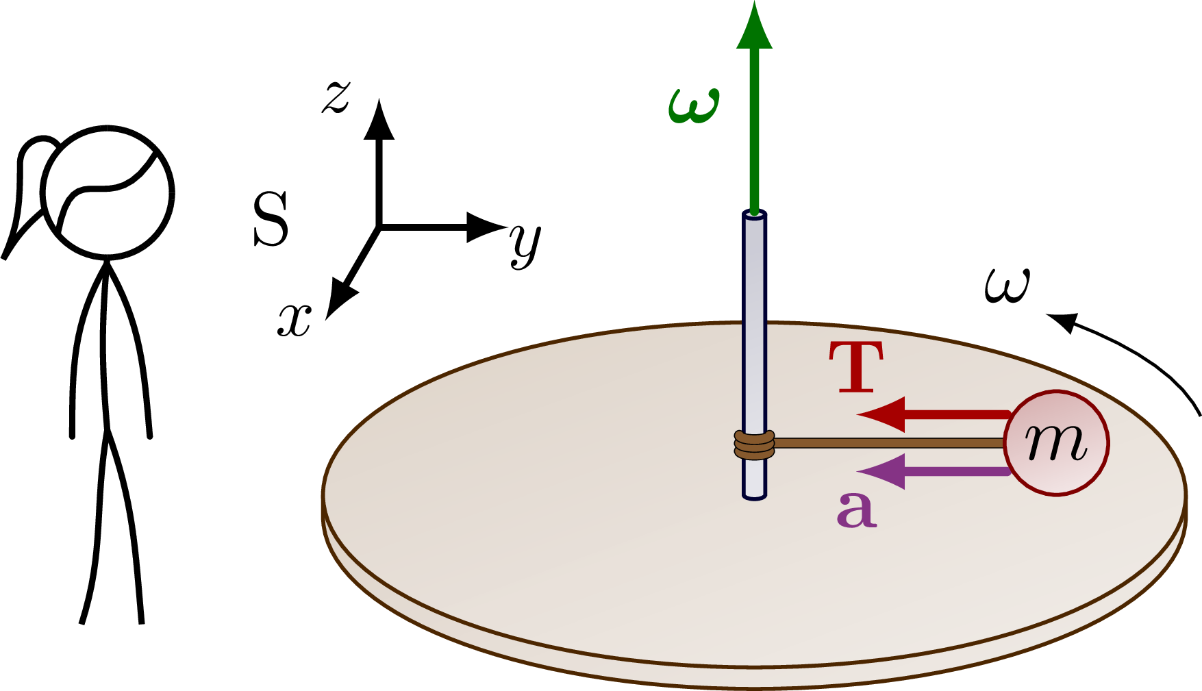
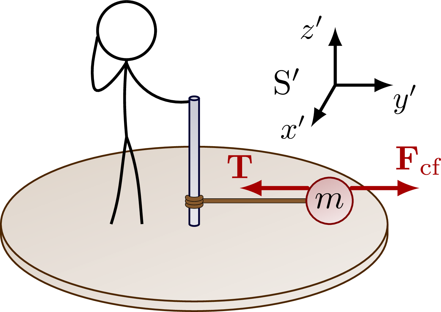
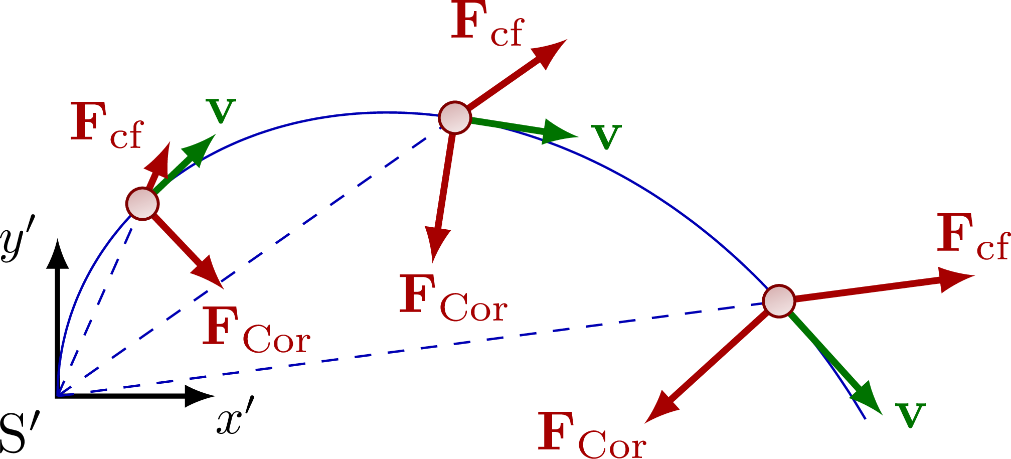
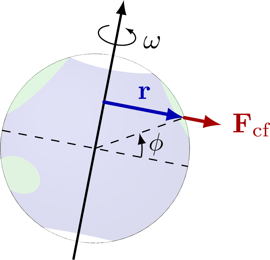
Rotating a reference frame, and pseudo forces (centrifugal & Coriolis), and derivation of the rotation matrix.


Edit and compile if you like:
% Author: Izaak Neutelings (September 2020)
\documentclass[border=3pt,tikz]{standalone}
\usepackage{amsmath}
\usepackage{tikz}
\usepackage{physics}
\usepackage[outline]{contour} % glow around text
\usetikzlibrary{calc}
\usetikzlibrary{decorations.markings}
\usetikzlibrary{angles,quotes} % for pic
\usetikzlibrary{arrows.meta} % for arrow size
\usetikzlibrary{bending} % for arrow head angle
\usetikzlibrary{decorations.pathmorphing} % for decorate random steps
\tikzset{>=latex} % for LaTeX arrow head
\usepackage{xcolor}
\contourlength{1.3pt}

\colorlet{xcol}{blue!70!black}
\colorlet{xcol'}{xcol!50!red}
\colorlet{vcol}{green!45!black}
\colorlet{acol}{red!50!blue!80!black!80}
\tikzstyle{rvec}=[->,very thick,xcol,line cap=round]
\tikzstyle{vvec}=[->,very thick,vcol,line cap=round]
\tikzstyle{avec}=[->,very thick,acol,line cap=round]
\colorlet{myred}{red!65!black}
\tikzstyle{force}=[->,myred,very thick,line cap=round]
\tikzstyle{mass}=[line width=0.5,draw=red!50!black,fill=red!50!black!10,rounded corners=1,
                  top color=red!50!black!30,bottom color=red!50!black!10,shading angle=20]
\tikzstyle{disk}=[line width=0.5,orange!30!black,fill=orange!40!black!10,
                  top color=orange!40!black!20,bottom color=orange!40!black!10,shading angle=20]
\tikzstyle{pole}=[line width=0.5,blue!20!black,fill=orange!20!black!10,
                  top color=blue!20!black!20,bottom color=blue!20!black!10,shading angle=20]
\tikzstyle{rope}=[brown!70!black,line width=1,line cap=round] %very thick
\tikzstyle{myarr}=[-{Latex[length=3,width=2,flex'=1]},thin]
\tikzstyle{mydashed}=[dash pattern=on 2pt off 1pt]
\def\rope#1{ \draw[rope,black,line width=1.4] #1; \draw[rope,line width=1.1] #1; }
\def\tick#1#2{\draw[thick] (#1) ++ (#2:0.1) --++ (#2-180:0.2)}
\newcommand\rightAngle[4]{
  \pgfmathanglebetweenpoints{\pgfpointanchor{#2}{center}}{\pgfpointanchor{#3}{center}}
  \coordinate (tmpRA) at ($(#2)+(\pgfmathresult+45:#4)$);
  %\draw[white,line width=0.6] ($(#2)!(tmpRA)!(#1)$) -- (tmpRA) -- ($(#2)!(tmpRA)!(#3)$);
  \draw[black] ($(#2)!(tmpRA)!(#1)$) -- (tmpRA) -- ($(#2)!(tmpRA)!(#3)$);
}


\begin{document}


% ROTATION
\def\L{3.1}     % axis lengths
\def\R{1.0*\L}  % position vector radial distance
\def\Rang{52}   % position vector angle
\def\ang{25}    % angle of the CM velocity
\begin{tikzpicture}
  \coordinate (O) at (0,0);
  \coordinate (X) at (1.05*\L,0);
  \coordinate (Y) at (0,1.05*\L);
  \coordinate (X') at (\ang:\L);
  \coordinate (Y') at (90+\ang:\L);
  \coordinate (R) at (\Rang:\R);
  \node[fill=blue!40!black,circle,inner sep=0.9] (R') at (R) {};
  \node[above right=-1] at (R') {P};
  \coordinate (Rx) at (0:{\R*cos(\Rang)});
  \coordinate (Ry) at (90:{\R*sin(\Rang)}); %($(Y)!(O)!(R)$);
  \coordinate (Rx') at (\ang:{\R*cos(\Rang-\ang)});
  \coordinate (Ry') at (90+\ang:{\R*sin(\Rang-\ang)});

  % AXES
  \draw[<->,very thick,xcol!70!black]
    (X) node[right=-1,xcol] {$x$} -- (O) node[below left=-3] {O} --
    (Y) node[left=-1,xcol] {$y$};
  \draw[<->,very thick,xcol'!70!black]
    (X') node[above=2,right=-2,xcol'] {$x'$} -- (O) --
    (Y') node[left=-2,xcol'] {$y'$};

  % POSITION VECTOR
  \draw[rvec,vvec,line cap=round] (O) -- (R') node[midway,left=2,above=1] {$\vb{r}$};
  \draw pic[-{Latex[length=3,width=2,flex'=1]},"$\theta=\omega t$"{scale=0.95,above=2,right},
            draw,angle radius=20,angle eccentricity=1] {angle=X--O--X'};

  % ANGLES
  \begin{scope}[xcol!70!black]
    \draw[dashed] (Ry) -- (R') -- (Rx);
    \tick{Rx}{90};
    \tick{Ry}{0};
    \rightAngle{R'}{Rx}{X}{0.25}
    \rightAngle{Y}{Ry}{R'}{0.25}
  \end{scope}
  \begin{scope}[xcol'!70!black]
    \draw[dashed] (Ry') -- (R') -- (Rx');
    \tick{Rx'}{90+\ang};
    \tick{Ry'}{\ang};
    \rightAngle{X'}{Rx'}{R'}{0.25}
    \rightAngle{Y'}{Ry'}{R'}{0.25}
  \end{scope}

\end{tikzpicture}


% ROTATION + angles
\begin{tikzpicture}
  \coordinate (Rx'') at (\ang:{\R*cos(\Rang)*cos(\ang)});     % projection of Rx on x' axis
  \coordinate (Ry'') at (90+\ang:{\R*sin(\Rang)*cos(\ang)});  % projection of Ry on y' axis
  \coordinate (Rx''') at ($(R')+(-90+\ang:{\R*sin(\Rang)*cos(\ang)})$); % projection of Rx on R-Rx' line
  \coordinate (Ry''') at ($(R')+(180+\ang:{\R*cos(\Rang)*cos(\ang)})$); % projection of Ry on R-Ry' linex

  % TRIANGLES
  \fill[xcol!70!black!10]
    (O) -- (Rx) -- (Rx'') -- cycle
    (O) -- (Ry) -- (Ry'') -- cycle;
  \fill[xcol'!70!black!10]
    (R) -- (Rx) -- (Rx''') -- cycle
    (R) -- (Ry) -- (Ry''') -- cycle;
  \node[fill=blue!40!black,circle,inner sep=0.9] at (R') {};
  \node[above right=-1] at (R') {P};

  % AXES
  \draw[<->,very thick,xcol!70!black]
    (X) node[right=-1,xcol] {$x$} -- (O) node[left=1,below=-1] {O} --
    (Y) node[left=-1,xcol] {$y$};
  \draw[<->,very thick,xcol'!70!black]
    (X') node[above=2,right=-2,xcol'] {$x'$} -- (O) --
    (Y') node[left=-2,xcol'] {$y'$};

  % POSITION VECTOR
  \draw[vvec,line cap=round] (O) -- (R'); %node[midway,left=2,above=1] {$\vb{r}$};
  \draw pic["$\theta$"{scale=0.9},
            draw,angle radius=20,angle eccentricity=1.22] {angle=X--O--X'};
  \draw pic["$\theta$"{scale=0.9},
            draw,angle radius=20,angle eccentricity=1.22] {angle=Y--O--Y'};
  \draw pic["$\theta$"{scale=0.9},
            draw,angle radius=17,angle eccentricity=1.30] {angle=Rx--R'--Rx'};
  \draw pic["$\theta$"{scale=0.9},
            draw,angle radius=17,angle eccentricity=1.30] {angle=Ry--R'--Ry'};

  % ANGLES
  \begin{scope}[xcol!80!black]
    \draw[dashed]
      (Ry) -- (R') node[midway,above=-1,scale=0.9] {$x$} --
      (Rx) node[midway,left=-1,scale=0.9] {$y$};
    \tick{Rx}{90};
    \tick{Ry}{0};
    \rightAngle{R'}{Rx}{X}{0.25}
    \rightAngle{Y}{Ry}{R'}{0.25}
  \end{scope}
  \begin{scope}[xcol'!80!black]
    \draw[dashed] (Ry') -- (R') -- (Rx''');
    \draw[dashed] (Ry) -- (Ry'');
    \draw[dashed] (Rx) -- (Rx'');
    \draw[dashed] (Rx) -- (Rx''');
    \draw[dashed] (Ry) -- (Ry''');
    \tick{Rx'}{90+\ang};
    \tick{Ry'}{\ang};
    \tick{Rx''}{90+\ang};
    \tick{Ry''}{\ang};
    \rightAngle{X'}{Rx'}{R'}{0.25}
    \rightAngle{Y'}{Ry'}{R'}{0.25}
    \rightAngle{Rx}{Rx''}{O}{0.25}
    \rightAngle{Ry}{Ry''}{O}{0.25}
    \rightAngle{Ry}{Ry'''}{R}{0.25}
    \rightAngle{Rx}{Rx'''}{R}{0.25}
  \end{scope}

  % LENGTHS
  %\node[xcol!70!black,above,scale=0.8] at ($(Ry)!0.5!(R)$) {$x$};
  \node[xcol!80!black!60,above,scale=0.8,rotate=\ang] at ($(O)!0.6!(Rx'')$) {$x\cos\theta$};
  \node[xcol'!80!black!60,right=1,below=-2,scale=0.8,rotate=\ang] at ($(Rx)!0.6!(Rx''')$) {\contour{white}{$y\sin\theta$}};
  %\node[xcol!80!black!60,below=4,scale=0.8,rotate=-90+\ang] at ($(O)!0.6!(Ry'')$) {$y\cos\theta$};
  \node[xcol'!80!black!60,below=-1,scale=0.8,rotate=-90+\ang] at ($(Ry)!0.6!(Ry''')$) {\contour{white}{$x\sin\theta$}};
  \draw[<->,xcol!80!black!60]
    ([shift={(180+\ang:0.3)}]O) -- ([shift={(180+\ang:0.3)}]Ry'')
    node[xcol!80!black!60,midway,scale=0.8,rotate=-90+\ang,fill=white,inner sep=0.5] {$y\cos\theta$};

\end{tikzpicture}


% STATIONARY REFERENCE FRAME - CENTRIFUGAL
\def\R{2}      % disk radius
\def\t{0.1}    % disk thickness
\def\p{0.05}   % pole radius
\def\P{1.3}    % pole height
\def\r{0.24}   % mass radius
\def\L{0.7*\R} % rope length
\def\H{2.0}    % human height
\begin{tikzpicture}

  % PERSON
  \coordinate (H) at (0,\H);
  \draw[thick,line cap=round]
    (H)++(-165:0.3) to[out=-140,in=60]++ (-130:0.3)
    to[out=65,in=-90,looseness=1.0]++ (80:0.45) to[out=90,in=120,looseness=1.4]++ (20:0.2); % pony tail
  \draw[thick,fill=white] (H) circle (0.3);
  \draw[thick,line cap=round] (H)++(-140:0.3) to[out=80,in=-120,looseness=1.8]++ (40:0.6); % hair
  \draw[thick] (H)++(-90:0.3) coordinate (N) to[out=-95,in=95]++ (0,-0.40*\H) coordinate (P);
  \draw[thick,line cap=round] (N)++(-95:0.03) to[out=-60,in=95]++ (0.10*\H,-0.4*\H) coordinate (RH);
  \draw[thick,line cap=round] (N)++(-95:0.03) to[out=-120,in=90]++ (-0.08*\H,-0.4*\H);
  \draw[thick] (P) to[out=-70,in=95] (0.08*\H,0);
  \draw[thick] (P) to[out=-100,in=72] (-0.06*\H,0);

  % AXIS
  \node (A) at (0.38*\H,0.94*\H) {S};
  \draw[<->,line width=0.9]
    (A)++(0.25*\H,0.28*\H) node[left,scale=0.9] {$z$} --++ (0,-0.3*\H) coordinate (O) --++
         (0.3*\H,0) node[below right=-3.5,scale=0.9] {$y$};
  \draw[->,line width=0.9] (O) --++ (-120:0.25*\H) node[left=-2,scale=0.9] {$x$};

  % DISK
  \begin{scope}[shift={(0.5*\H+\R,0.3*\H)}]
    \coordinate (T) at (0,\r);
    \draw[disk] (-\R,0) --++ (0,-\t) arc(180:360:{\R} and {0.4*\R}) --++ (0,\t);
    \draw[disk] (0,0) ellipse({\R} and {0.4*\R});
    \rope {(T) --++ (\L,0) coordinate (M)};
    \draw[pole] (-\p,\P) --++ (0,-\P) arc(180:360:{\p} and {0.4*\p}) --++ (0,\P);
    \draw[pole] (0,\P) ellipse({\p} and {0.4*\p});
    \rope {(-1.4*\p,0.85*\r) arc(180:360:{1.4*\p} and {0.4*\p})}
    \rope {(-1.4*\p,1.00*\r) arc(180:360:{1.4*\p} and {0.4*\p})}
    \rope {(-1.4*\p,1.15*\r) arc(180:360:{1.4*\p} and {0.4*\p})}
    \draw[force] (M)++(150:1.1*\r) --++ (-0.5*\L,0) node[above=-1] {$\vb{T}$};
    \draw[avec] (M)++(210:1.1*\r) --++ (-0.5*\L,0) node[right=0,below=-1] {$\vb{a}$}; %_\mathrm{cm}
    \draw[mass] (M) circle(\r) node {$m$};
    \draw[->] (10:1.05*\R) arc(10:50:{1.05*\R} and {0.4*\R}) node[above left=-2] {$\omega$};
    \draw[vvec] (0,\P+0.014) --++ (0,0.7*\L) node[midway,left] {$\vb*\omega$};
  \end{scope}

\end{tikzpicture}


% MOVING REFERENCE FRAME - CENTRIFUGAL
\begin{tikzpicture}

  % DISK
  \coordinate (T) at (0,\r);
  \draw[disk] (-\R,0) --++ (0,-\t) arc(180:360:{\R} and {0.4*\R}) --++ (0,\t);
  \draw[disk] (0,0) ellipse({\R} and {0.4*\R});

  % PERSON
  \draw[thick,fill=white] (-0.35*\R,\H) circle (0.15*\H) coordinate (H);
  \draw[thick] (H)++(-90:0.15*\H) coordinate (N) to[out=-95,in=95]++ (0,-0.40*\H) coordinate (P);
  \draw[thick,line cap=round] (N)++(-95:0.03) to[out=-70,in=190]++ (0.34*\H,-0.20*\H);
  \draw[thick,line cap=round] (N)++(-95:0.03) to[out=-120,in=-80]++ (-0.17*\H,-0.12*\H) to[out=100,in=-100]++ (0.02*\H,0.25*\H);
  \draw[thick] (P) to[out=-70,in=95] ($(H)+(0.08*\H,-\H)$);
  \draw[thick] (P) to[out=-100,in=72] ($(H)+(-0.08*\H,-\H)$);

  % POLE + MASS
  \rope {(T) --++ (\L,0) coordinate (M)};
  \draw[pole] (-\p,\P) --++ (0,-\P) arc(180:360:{\p} and {0.4*\p}) --++ (0,\P);
  \draw[pole] (0,\P) ellipse({\p} and {0.4*\p});
  \rope {(-1.4*\p,0.85*\r) arc(180:360:{1.4*\p} and {0.4*\p})}
  \rope {(-1.4*\p,1.00*\r) arc(180:360:{1.4*\p} and {0.4*\p})}
  \rope {(-1.4*\p,1.15*\r) arc(180:360:{1.4*\p} and {0.4*\p})}
  \draw[force] (M)++(150:1.1*\r) --++ (-0.5*\L,0) node[above=-1] {$\vb{T}$};
  \draw[force] (M)++(30:1.1*\r) --++ (0.5*\L,0) node[above=0] {$\vb{F}_\mathrm{cf}$};
  \draw[mass] (M) circle(\r) node {$m$};

  % AXIS
  \node (A) at (57:0.88*\R) {S$'$};
  \draw[<->,line width=0.9]
    (A)++(0.25*\H,0.28*\H) node[left,scale=0.9] {$z'$} --++ (0,-0.3*\H) coordinate (O) --++
         (0.3*\H,0) node[below right=-3.5,scale=0.9] {$y'$};
  \draw[->,line width=0.9] (O) --++ (-120:0.25*\H) node[left=-2,scale=0.9] {$x'$};

\end{tikzpicture}


% STATIONARY REFERENCE FRAME - CORIOLIS
\def\R{2}       % disk radius
\def\r{0.1}     % mass radius
\def\v{0.35*\R} % mass velocity
\def\x{0.48}    % mass position (fraction of \R)
\def\ang{50}    % angle displacement
\begin{tikzpicture}
  \coordinate (O) at (0,0);
  \coordinate (T) at (0,\r);
  \coordinate (M) at (90:0.45*\R);
  \coordinate (S) at (-145:1.6*\R);
  \coordinate (B) at (90+\x*\ang:0.88*\R);

  % DISK & DOTS
  \draw[disk] (O) circle(\R);
  \fill[myred!20] (90:0.88*\R) circle(0.05*\R);
  \fill[myred] (90+\x*\ang:0.88*\R) circle(0.05*\R);
  \fill[myred!20] (90+\ang:0.88*\R) circle(0.05*\R);
  \draw[xcol,->] (92:0.88*\R) arc(92:88+\ang:0.88*\R);

  % MASS
  \draw[<->,black!25,line width=0.9]
    (0,0.35*\R) |-++ (0.35*\R,-0.35*\R);
  \draw[xcol] (O) --++ (90:1.1*\R);
  \draw[vvec] (M) --++ (90:\v) node[below right] {$\vb{v}$};
  \draw[mass] (M) circle(\r) node[right=1] {$m$};
  \draw[->] (10:1.1*\R) arc(10:35:1.1*\R) node[left=2,above=0] {$\omega$};

  % AXIS
  \node[left=2] at (S) {S};
  \draw[<->,line width=0.9]
    (S)++(0,0.38*\R) node[left,scale=0.9] {$y$} |-++
         (0.35*\R,-0.35*\R) node[below right=-3,scale=0.9] {$x$};

  % AXIS S'
  \draw[<->,line width=0.9]
    (90+\x*\ang:0.35*\R) node[below left=-2,scale=0.9] {$y'$} -- (0,0) --
    (\x*\ang:0.35*\R) node[above=3,right=-2,scale=0.9] {$x'$};
  \node[below=1] at (O) {A};
  \node[right=1,below=1] at (B) {B};

\end{tikzpicture}


% MOVING REFERENCE FRAME - CORIOLIS
\begin{tikzpicture}
  \def\v{0.40*\R}        % mass velocity
  \def\vv{2.0}           % velocity for plot
  \def\FC{0.30*\R}       % Coriolis force
  \def\om{180/pi}        % angular frequency omega
  \def\tmax{1.10}        % maximum t
  \def\xt{0.98*\x*\tmax} % mass position
  \coordinate (T) at (0,\r);
  \coordinate (S) at (-145-\ang:1.6*\R);
  \coordinate (M) at ({\vv*\xt*sin(\om*\xt)},{\vv*\xt*cos(\om*\xt)});
  \coordinate (V) at ({\v*sin(\om*\xt)+\v*\xt*cos(\om*\xt)},{\v*cos(\om*\xt)-\v*\xt*sin(\om*\xt)});
  \coordinate (F) at ({\FC*cos(\om*\xt)-\FC*\xt*sin(\om*\xt)},{-\FC*sin(\om*\xt)-\FC*\xt*cos(\om*\xt)});

  % DISK & DOTS
  \draw[disk] (0,0) circle(\R);
  \fill[myred] (90:0.88*\R) circle(0.05*\R);

  % AXIS
  \draw[xcol,dashed] (0,0) --++ (90:1.1*\R);
  \node[below left=-1] at (0,0) {S$'$};
  \draw[<->,line width=0.9]
    (0,0.35*\R) node[left,scale=0.9] {$y'$} |-++
    (0.35*\R,-0.35*\R) node[below right=-3.5,scale=0.9] {$x'$};

  % MASS
  \draw[xcol,samples=50,smooth,variable=\t,domain=0:\tmax]
    plot({\vv*\t*sin(\om*\t)},{\vv*\t*cos(\om*\t)});
  %\fill[myred] (90-\ang:0.88*\R) circle(0.05); % check
  \draw[vvec] (M) --++ (V) node[above=3,left=0] {$\vb{v}$};
  \draw[force] (M) --++ (F) node[right=-1] {$\vb{F}_\mathrm{Cor}$};
  \draw[mass] (M) circle(\r) node[left=4,above=2] {$m$};

  % AXIS
  \node[left=2] at (S) {S};
  \draw[<->,black!25,line width=0.9]
    (-145:1.6*\R)++(0,0.38*\R) node[left,scale=0.9] {$y$} |-++
                   (0.35*\R,-0.35*\R) node[below right=-3,scale=0.9] {$x$};
  \draw[<->,line width=0.9]
    (S)++(90-\ang:0.38*\R) node[left=3,scale=0.9] {$y$} --++ (-90-\ang:0.38*\R) --++
         (-\ang:0.38*\R) node[below right=-3,scale=0.9] {$x$};
  \draw[->] (-165:1.55*\R) arc(-150:-210:0.6*\R) node[midway,left=0] {$\omega$};

\end{tikzpicture}


% CENTRIFUGAL + CORIOLIS
\begin{tikzpicture}
  \def\vv{3.2}         % velocity for plot
  \def\v{0.25*\R}      % velocity size
  \def\Fc{0.40*\R}     % centrifugal force
  \def\FC{0.30*\R}     % Coriolis force
  \def\om{180/pi}      % angular frequency omega
  \def\tmax{1.6}       % maximum t
  \def\ta{0.26*\tmax} % mass position A
  \def\tb{0.60*\tmax} % mass position B
  \def\tc{0.90*\tmax} % mass position C
  \def\vRM#1{{\vv*#1*sin(\om*#1)},{\vv*#1*cos(\om*#1)}}
  \def\vvc#1{{\v*sin(\om*#1)+\v*#1*cos(\om*#1)},{\v*cos(\om*#1)-\v*#1*sin(\om*#1)}}
  \def\vFc#1{{\Fc*#1*sin(\om*#1)},{\Fc*#1*cos(\om*#1)}}
  \def\vFC#1{{\FC*cos(\om*#1)-\FC*#1*sin(\om*#1)},{-\FC*sin(\om*#1)-\FC*#1*cos(\om*#1)}}
  \def\vang#1{atan2({\v*cos(\om*#1)-\v*#1*sin(\om*#1)},{\v*sin(\om*#1)+\v*#1*cos(\om*#1)})}
  \coordinate (O) at (0,0);
  \coordinate (MA) at (\vRM{\ta});
  \coordinate (MB) at (\vRM{\tb});
  \coordinate (MC) at (\vRM{\tc});
  %\node[mass,circle,inner sep=2] (MA) at (\vRM{\ta}) {};
  %\node[mass,circle,inner sep=2] (MB) at (\vRM{\tb}) {};
  %\node[mass,circle,inner sep=2] (MC) at (\vRM{\tc}) {};

  % AXIS
  \node[below left=-1] at (0,0) {S$'$};
  \draw[<->,line width=0.9]
    (0,0.5*\R) node[left,scale=0.9] {$y'$} |-++
    (0.5*\R,-0.5*\R) node[below right=-3.5,scale=0.9] {$x'$};

  % PLOT
  \draw[xcol,samples=50,smooth,variable=\t,domain=0:\tmax]
    plot({\vv*\t*sin(\om*\t)},{\vv*\t*cos(\om*\t)});
  \draw[dashed,xcol] (O) -- (MA);
  \draw[dashed,xcol] (O) -- (MB);
  \draw[dashed,xcol] (O) -- (MC);

  % MASS A
  \draw[vvec]  (MA)++({\vang{\ta}}:\r) --++ (\vvc{\ta}) node[right=1,above=-2] {$\vb{v}$};
  \draw[force] (MA)++(90-\om*\ta:\r) --++ (\vFc{\ta}) node[above=3,left=0] {$\vb{F}_\mathrm{cf}$};
  \draw[force] (MA)++({\vang{\ta}-90}:\r) --++ (\vFC{\ta}) node[right=6,below=-1] {\contour{white}{$\vb{F}_\mathrm{Cor}$}};
  \draw[mass]  (MA) circle(\r); %node[left=4,above=2] {$m$};

  % MASS B
  \draw[vvec]  (MB)++({\vang{\tb}}:\r) --++ (\vvc{\tb}) node[right=-2] {$\vb{v}$};
  \draw[force] (MB)++(90-\om*\tb:\r) --++ (\vFc{\tb}) node[above=3,left=3] {$\vb{F}_\mathrm{cf}$};
  \draw[force] (MB)++({\vang{\tb}-90}:\r) --++ (\vFC{\tb}) node[right=4,below=-2] {$\vb{F}_\mathrm{Cor}$};
  \draw[mass]  (MB) circle(\r);

  % MASS C
  \draw[vvec]  (MC)++({\vang{\tc}}:\r) --++ (\vvc{\tc}) node[right=-2] {$\vb{v}$};
  \draw[force] (MC)++(90-\om*\tc:\r) --++ (\vFc{\tc}) node[above=-1] {$\vb{F}_\mathrm{cf}$};
  \draw[force] (MC)++({\vang{\tc}-90}:\r) --++ (\vFC{\tc}) node[below=2,left=-5] {$\vb{F}_\mathrm{Cor}$};
  \draw[mass]  (MC) circle(\r);

\end{tikzpicture}


% EARTH + CENTRIFUGAL
\contourlength{0.7pt}
\begin{tikzpicture}
  \def\E{1.2}
  \def\ang{30} % latidude
  \coordinate (O) at (0,0);

  % EARTH
  %\draw[dashed,rotate=-11] (0,-1.3*\E) -- (0,1.45*\E);
  \fill[blue!70!black!70] (0,0) circle (1.2);
  \draw[very thin,ball color=blue!70!black!40,fill opacity=0.2] (0,0) circle (\E);
  \begin{scope}[rotate=-11]
    \draw[-{Latex[length=3,width=2,flex'=1]}]
      (0,1.22*\E)++(120:{0.2*\E} and 0.1*\E) arc(120:430:{0.2*\E} and 0.1*\E)
      node[pos=0.7,right=0] {$\omega$};
    \clip (0,0) circle (\E);
    \fill[white] (0,\E) ellipse ({0.6*\E} and {0.15*\E});
    \fill[white] (0,-\E) ellipse ({0.8*\E} and {0.08*\E});
    \fill[green!70!black!60,rotate=-30] (160:1.1*\E) ellipse ({0.2*\E} and {0.8*\E});
    \fill[green!70!black!60,rotate=40] (-10:1.14*\E) ellipse ({0.2*\E} and {0.9*\E});
    \fill[green!60!black!60,very thick,rotate=-20] % Australia
      (230:0.86*\E) ellipse ({0.25*\E} and {0.18*\E});
    \fill[fill=white,fill opacity=0.8] (0,0) circle (\E);
  \end{scope}
  \begin{scope}[rotate=-11]
    %\draw[dashed] (-\E,0) to[out=-20,in=-160] (\E,0);
    %\draw[->,thick] (-1.2*\E,0) -- (1.2*\E,0);
    \draw[dashed] (-\E,0) -- (\E,0) coordinate (X);
    \draw[dashed] (O) -- (\ang:\E) coordinate (R);
    \draw[->,thick] (0,-1.2*\E) -- (0,1.6*\E);
    \draw[rvec] (0,{\E*sin(\ang)}) -- (R) node[midway,above=0] {$\vb{r}$};
    \draw[force] (R) --++ (0.4*\E,0) node[right] {$\vb{F}_\mathrm{cf}$};
    \draw pic[->,"$\phi$"{scale=0.9}, %{Latex[length=3,width=2,flex'=1]}
              draw,angle radius=17,angle eccentricity=1.3] {angle=X--O--R};
  \end{scope}

\end{tikzpicture}


% EARTH + CORIOLIS
\contourlength{0.7pt}
\begin{tikzpicture}
  \def\E{1.2}
  \coordinate (O) at (0,0);

  % EARTH
  \draw[dashed,rotate=-11] (0,-1.3*\E) -- (0,1.45*\E);
  \fill[blue!70!black!70] (0,0) circle (1.2);
  \draw[very thin,ball color=blue!70!black!40,fill opacity=0.2] (0,0) circle (\E);
  \begin{scope}[rotate=-11]
    \draw[-{Latex[length=3,width=2,flex'=1]}] (0,1.22*\E)++(120:{0.2*\E} and 0.1*\E) arc(120:430:{0.2*\E} and 0.1*\E);
    \clip (0,0) circle (\E);
    \fill[white] (0,\E) ellipse ({0.6*\E} and {0.15*\E});
    \fill[white] (0,-\E) ellipse ({0.8*\E} and {0.08*\E});
    \fill[green!70!black!60,rotate=-30] (160:1.1*\E) ellipse ({0.2*\E} and {0.8*\E});
    \fill[green!70!black!60,rotate=40] (-10:1.14*\E) ellipse ({0.2*\E} and {0.9*\E});
    \fill[green!60!black!60,very thick,rotate=-20] % Australia
      (230:0.86*\E) ellipse ({0.25*\E} and {0.18*\E});
    \draw[dashed] (-\E,0) to[out=-20,in=-160] (\E,0);

    % CORIOLIS
    \draw[myred,mydashed,very thin] (0,-0.1*\E) coordinate (NS) --++ (0, 0.70*\E) coordinate (NN);
    \draw[myred,mydashed,very thin] (0,-0.3*\E) coordinate (SN) --++ (0,-0.60*\E) coordinate (SS);
    \draw[myred,mydashed,very thin] (-0.4*\E,0.32*\E) coordinate (NW) to[out=-20,in=-160]++ (0.8*\E,0) coordinate (NE);
    \draw[myred,mydashed,very thin] (-0.4*\E,-0.53*\E) coordinate (SW) to[out=-20,in=-160]++ (0.8*\E,0) coordinate (SE);
    \draw[myarr,red] (NN) to[out=-90,in=  50]++ (-110:0.35*\E); % northern hemisphere
    \draw[myarr,red] (NS) to[out= 90,in=-120]++ (  70:0.35*\E);
    \draw[myarr,red] (SN) to[out=-90,in= 130]++ ( -65:0.30*\E); % southern hemisphere
    \draw[myarr,red] (SS) to[out= 90,in= -60]++ ( 110:0.30*\E);
    \draw[myarr,red] (NE) to[out=200,in= -40]++ (170:0.38*\E); % northern hemisphere
    \draw[myarr,red] (NW) to[out=-20,in= 140]++ (-30:0.42*\E);
    \draw[myarr,red] (SE) to[out=200,in=  40]++ (210:0.42*\E); % southern hemisphere
    \draw[myarr,red] (SW) to[out=-20,in=-140]++ ( 10:0.38*\E);
  \end{scope}

  \node at (108-11:1.2*\E) {N};
  \node at (180-11:1.2*\E) {W};
  \node at (   -11:1.2*\E) {E};
  \node at (-98-11:1.2*\E) {S};

\end{tikzpicture}


\end{document}
Click to download: reference_frame_rotational.tex • reference_frame_rotational.pdf
Open in Overleaf: reference_frame_rotational.tex


Hello,
Last question (I promise).
I am using one of your Earth diagrams to do a diagram of the seasons (have a Sun in the middle and the tilted Earth in four different position).
I tried to duplicate the diagram by brute force, but I was unable to do it. I have been doing some research, but can’t seem to find it. Is there a simple way to duplicate and translate pictures in tikz, so that I can make the four Earths in the same slide (I am using for beamer)?
If I can’t do it, I will do each season on a different slide, as changing the position of a yellow circle fits better with my teaching time constraints… hehehe
Again, thank you,
Wagner.
Again, thank you,
Hello,
Last question (I promise).
I am using one of your Earth diagrams to do a diagram of the seasons (have a Sun in the middle and the tilted Earth in four different position).
I tried to duplicate the diagram by brute force, but I was unable to do it. I have been doing some research, but can’t seem to find it. Is there a simple way to duplicate and translate pictures in tikz, so that I can make the four Earths in the same slide (I am using for beamer)?
If I can’t do it, I will do each season on a different slide, as changing the position of a yellow circle fits better with my teaching time constraints… hehehe
Again, thank you,
Wagner.
Hi Wagner,
I am not 100% sure what you need, but you probably need to define some macro. There are two options I often use myself:
\deffor simple things, and\picfor things that need a more functionality and complexity. They both can take arguments depending on how you define it. The advantage ofpicis that you can also draw some predefined picture at a give coordinate (what you’d need for translating a picture of Earth), and you can transform it (rotate, scale, etc.). It also allows styling, default arguments, etc.Have a look at Chapter 18 in the manual for more on
pic: https://tikz.dev/tikz-pics You can also find more examples on this site with the def and pic tags.In your case you just need something like the polar angle to define the Earth’s position, right? You can play around with the following example yourself:
\documentclass[border=3pt,tikz]{standalone}
\tikzset{
  >=latex, % for LaTeX arrow head
  pics/myarrow/.style={ % argument #1 = polar angle
    code={
      \draw[->,ultra thick,red] (0,0) -- (#1:1.5);
    }
  },
}
\def\drawarrow#1{ % macro
  \draw[->,ultra thick,blue] (0,0) -- (#1:1.5);
}
\begin{document}

% MACRO using \def
\begin{tikzpicture}
  \draw[ultra thin] (-2,-2) grid (2,2);
  \foreach \ang in {30,60,...,360}{ % loop over polar angle
    \drawarrow{\ang}
  }
\end{tikzpicture}

% MACRO using \pic
\begin{tikzpicture}
  \draw[ultra thin] (-2,-2) grid (2,2);
  \foreach \ang in {30,60,...,360}{ % loop over polar angle
    \pic at (0,0) {myarrow=\ang};
  }
\end{tikzpicture}

\end{document}
In beamer, there are several ways to hide/show TikZ pictures in slide transitions. I am not an expert, so you need to dig a bit deeper yourself if you want something different (e.g. read this StackOverflow thread, or see this post with the SM particles):
\documentclass[aspectratio=169]{beamer}
\usepackage{tikz}
\usetikzlibrary{overlay-beamer-styles} % for alt=<...>{style}{default}

\tikzset{
  % https://tex.stackexchange.com/questions/88251/tikz-spy-and-beamer-uncover
  >=latex, % for LaTeX arrow head
  visible on/.style={alt={#1{}{invisible}}},
  pics/myarrow/.style={ % argument #1 = polar angle
    code={
      \draw[->,ultra thick,red] (0,0) -- (#1:1.5);
    }
  },
}

\begin{document}

\begin{frame}[fragile]
  \frametitle{An arrow}
  \begin{columns}

    % ARROW
    \column{0.49\linewidth}
    \centering
    \begin{tikzpicture}
      \draw[ultra thin] (-2,-2) grid (2,2);
      \pic[visible on=<{1,5-}>] at (0,0) {myarrow=0};
      \pic[visible on=<{2,5-}>] at (0,0) {myarrow=90};
      \pic[visible on=<{3,5-}>] at (0,0) {myarrow=180};
      \pic[visible on=<{4,5-}>] at (0,0) {myarrow=270};
    \end{tikzpicture}

    % TEXT
    \column{0.48\linewidth}
    \begin{itemize}
      \item<1-> Arrow 1 with $0^\circ$.
      \item<2-> Arrow 2 with $90^\circ$.
      \item<3-> Arrow 3 with $180^\circ$.
      \item<4-> Arrow 4 with $270^\circ$.
      \item<5-> All arrows again.
    \end{itemize}

  \end{columns}
\end{frame}

\end{document}
A very quick ‘n dirty Earth going around the sun is below:
\documentclass[border=3pt,tikz]{standalone}

\def\angE{23} % Earth axis tilt
\def\RE{0.4} % Earth radius
\def\ROx{3.0} % orbit horizontal radius
\def\ROy{0.9} % orbit vertical radius
\tikzset{
  orbit/.style={dashed,black!50},
  pics/earth/.style={ % Earth in orbit (argument #1 = polar angle)
    code={
      \coordinate (E) at (#1:{\ROx} and {\ROy});
      \draw[orbit] % orbit (back)
        (0,0) ellipse({\ROx} and {\ROy});
      \draw[orange!80!yellow!80,fill=orange!50!yellow!40] % Sun
        (0,0) circle (0.5*\ROy);
      \draw[fill=blue!70!cyan!80] % Earth
        (E) circle(\RE);
      \draw[dashed,line cap=round] % tilted axis
        (E)++(90-\angE:1.1*\RE) --++ (-90-\angE:2.25*\RE);
    }
  },
}

\begin{document}

% EARTH in orbit
\foreach \ang in {0,90,...,270}{ % loop over Earth position (polar angle)
\begin{tikzpicture}
  \pic at (0,0) {earth=\ang};
\end{tikzpicture}}

\end{document}
However, if you want to have overlapping pictures in the right order (e.g. Sun in front or behind the Earth), things can become quite messy quick, and need a lot of hacks and finetuning. Maybe it’s better to define a macro for just the Earth, so you draw it in the right order and at the right position yourself:
\documentclass[border=3pt,tikz]{standalone}

\def\angE{23} % Earth axis tilt
\def\RE{0.4} % Earth radius
\def\ROx{3.0} % orbit horizontal radius
\def\ROy{0.9} % orbit vertical radius
\tikzset{
  orbit/.style={dashed,black!50},
  pics/earth/.style={ % Earth in orbit (argument #1 = polar angle)
    code={
      \draw[fill=blue!70!cyan!80] % Earth
        (0,0) circle(\RE);
      \draw[dashed,line cap=round] % tilted axis
        (E)++(90-\angE:1.1*\RE) --++ (-90-\angE:2.25*\RE);
    }
  },
}

\begin{document}

% EARTH in orbit
\foreach \ang in {0,90,...,270}{ % loop over Earth position (polar angle)
\begin{tikzpicture}
  \coordinate (E) at (\ang:{\ROx} and {\ROy});
  \draw[orbit] % orbit
    (0,0) ellipse({\ROx} and {\ROy});
  \draw[orange!80!yellow!80,fill=orange!50!yellow!40] % Sun
    (0,0) circle (0.5*\ROy);
  \pic at (E) {earth=\ang};
\end{tikzpicture}}

\end{document}
Hope that helps,
Izaak
Hello Izaak,
Thank you so much for your diagrams. I did something like that for now, in a quick and dirty way, as you said, but I like your diagram so much that I was attempting to reproduce something like this:
https://faculty.kutztown.edu/courtney/blackboard/physical/21seasons/seasons1.jpg
This is to attempt to make it more visual how the Sun is directly opposite to the Equator during equinoxes and opposite to the tropics during solstice.
The quick and dirty way worked for now, but I I am still going to get this right! heheheeh
Again, thank you so much for your input! It is greatly appreciated!
Ah, I see. In that case try something like this:
% Author: Izaak Neutelings (January 2024)
\documentclass[border=3pt,tikz]{standalone}
\usetikzlibrary{arrows.meta,bending} % for arrow head size
\usetikzlibrary{calc} % for calculating coordinates

% FADINGS
\usetikzlibrary{fadings}
\begin{tikzfadingfrompicture}[name=halo]
  \shade[inner color=transparent!0,outer color=transparent!100]
    (0,0) circle (0.9);
\end{tikzfadingfrompicture}

% COLORS
\usepackage{xcolor}
\colorlet{water}{blue!70!cyan!80}
\colorlet{shadow}{water!60!black}

% STYLES & MACROS
\def\angE{23} % Earth axis tilt
\def\RE{0.4} % Earth radius
\def\ROx{3.0} % orbit horizontal radius
\def\ROy{0.9} % orbit vertical radius
\tikzset{
  >=latex, % for LaTeX arrow head
  orbit/.style={-{latex[scale=0.8,bend]},black!75}, %dashed
  altitude/.style={ultra thin,dash pattern=on 2pt off 1pt,opacity=0.8}, %dashed
  note/.style={red!90!black,align=center,scale=0.3},
  mysmallarrow/.style={-{Latex[length=3,width=2,bend]},red,line width=0.4,line cap=round},
  pics/earth/.style={ % Earth in orbit (argument #1 = polar angle)
    code={
      \coordinate (-O) at (#1:{\ROx} and {\ROy});
        \begin{scope}[shift={(-O)}]
        \draw[black!80,line cap=round] % tilted axis
          (0,0)++(90-\angE:1.24*\RE) coordinate(-N) % north
          --++ (-90-\angE:2.40*\RE) coordinate (-S); % south
        %\fill[water] (0,0) circle(\RE); % Earth fill (even)
        \begin{scope} % create bright spot shifted towards sun
          \clip (0,0) circle(\RE);
          \shade[inner color=water!50,outer color=water!80!black]
            (#1-180:{0.7*\RE} and {0.2*\RE}) circle(1.7*\RE);
        \end{scope}
        \fill[shadow] % Earth shadow
          \ifnum #1=0 (90:\RE) arc(90:-90:\RE) \fi % right shadow
          \ifnum #1=180 (90:\RE) arc(90:270:\RE) \fi % left shadow
          \ifnum #1=270 (0,0) circle(\RE) \fi; % full shadow
        \draw[rotate=-\angE,altitude,solid] % equator
          (-\RE,0) to[out=-12,in=-168] (\RE,0);
        \foreach \i [evaluate={\y=0.35*\i*\RE;\x=sqrt(\RE*\RE-\y*\y);}] in {1,2}{
          \draw[rotate=-\angE,altitude] % altitude lines
            (-\x,\y) to[out=-12,in=-168] (\x,\y)
            (-\x,-\y) to[out=-12,in=-168] (\x,-\y);
        }
        \draw[black,very thin] (0,0) circle(\RE); % Earth outline
        \draw[mysmallarrow] % indicate rotation
          (90-\angE:1.24*\RE)++(180:{0.14} and {0.1}) arc(180:330:{0.15} and {0.1});
      \end{scope}
    }
  }
}

\begin{document}

% EARTH in orbit
\begin{tikzpicture}
  \coordinate (O) at (0,0);
  \coordinate (S) at (0.02*\ROx,0); % sun (slightly shifted to focus, eccentricity ~ 0.02)
  \foreach \i [evaluate={\anga=(\i-1)*90+(mod(\i,2)==0?15:35)}] in {1,...,4}{
    \draw[orbit] % orbit
      (\anga:{\ROx} and {\ROy}) arc(\anga:\anga+40:{\ROx} and {\ROy});
  }
  \pic (E90) at (O) {earth=90}; % draw behind sun
  \fill[path fading=halo,orange!80!yellow!80] % solar halo/corona
    (S) circle (2.2*\RE);
  \draw[very thin,orange!80!yellow!80,fill=orange!50!yellow!40] % Sun
    (S) circle (1.5*\RE);
  \foreach \ang in {0,180,270}{
    \pic (E\ang) at (O) {earth=\ang}; % draw in front of sun
  }
  \node[note,above=3pt] at (E180-N) {June 21\\A};
  \node[note,below=2pt] at (E270-S) {B\\September 22};
  \node[note,above=3pt] at (E0-N) {December 21\\C};
  \node[note,above=3pt] at (E90-N) {March 21\\D};
\end{tikzpicture}

\end{document}
Note that if you define some coordinate
(-X)inside apiccode block, and you name your\pic (P) ..., you can reuse it later as(P-X), which is handy here to manually place labels at the north or south pole. Alternatively, you could program the label inside the Earthpic, and take a the text as a second argument.Also note that I used a bit of a hack with
\ifnum <condition> <do this>where the condition is some comparison between integers, to distinguish special cases, but this is already quite some finetuning.\else <do otherwise> \fi
One day, when it is maybe too late because of AI, I will be as good as you on tikz!!
Thank you so much!!!! I really appreciate it!
I will attempt to change the code to correct for the Sunlight on Earth during the solstices, but it shouldn’t be too much of a problem! 🙂
Fantastic! Again, thank you! 🙂
\fill[shadow,rotate=-\angE] % Earth shadow
\ifnum #1=0 (113:\RE) arc(113:-66:\RE) \fi % right shadow
\ifnum #1=180 (113:\RE) arc(113:293:\RE) \fi % left shadow
\ifnum #1=270 (0,0) circle(\RE) \fi; % full shadow
To correct for the shadows! 🙂
No problem!
Thank you for your correction, I was more paying attention to the styling than the physics I guess… :p
I will edit the code in my previous answer, and correct it as follows:
        \fill[shadow] % Earth shadow
          \ifnum #1=0 (90:\RE) arc(90:-90:\RE) \fi % right shadow
          \ifnum #1=180 (90:\RE) arc(90:270:\RE) \fi % left shadow
          \ifnum #1=270 (0,0) circle(\RE) \fi; % full shadow
By just removing
rotate=-\angEfrom the options in\fill, you do not have to finetune & hardcode the angles as a function of\angE=23.Hello Izaak,
Please, do let me know if you can help with the question above (If there is an easy way to translate the same image of the the tilted Earth to 4 different positions). I have been reading extensively about tikz, your diagrams have been an amazing lesson!
Again, thank you,
Wagner.