AC circuit plots

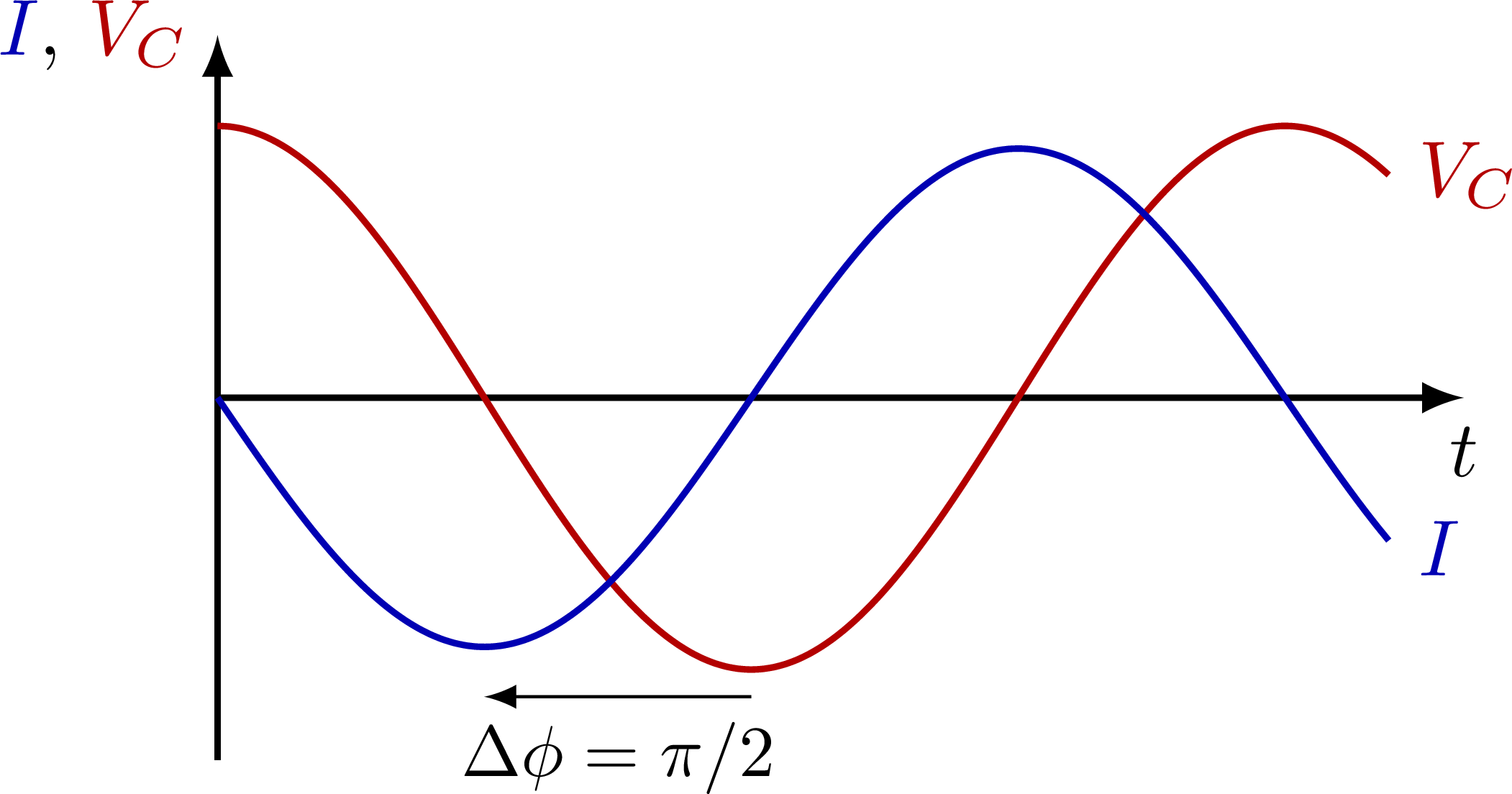
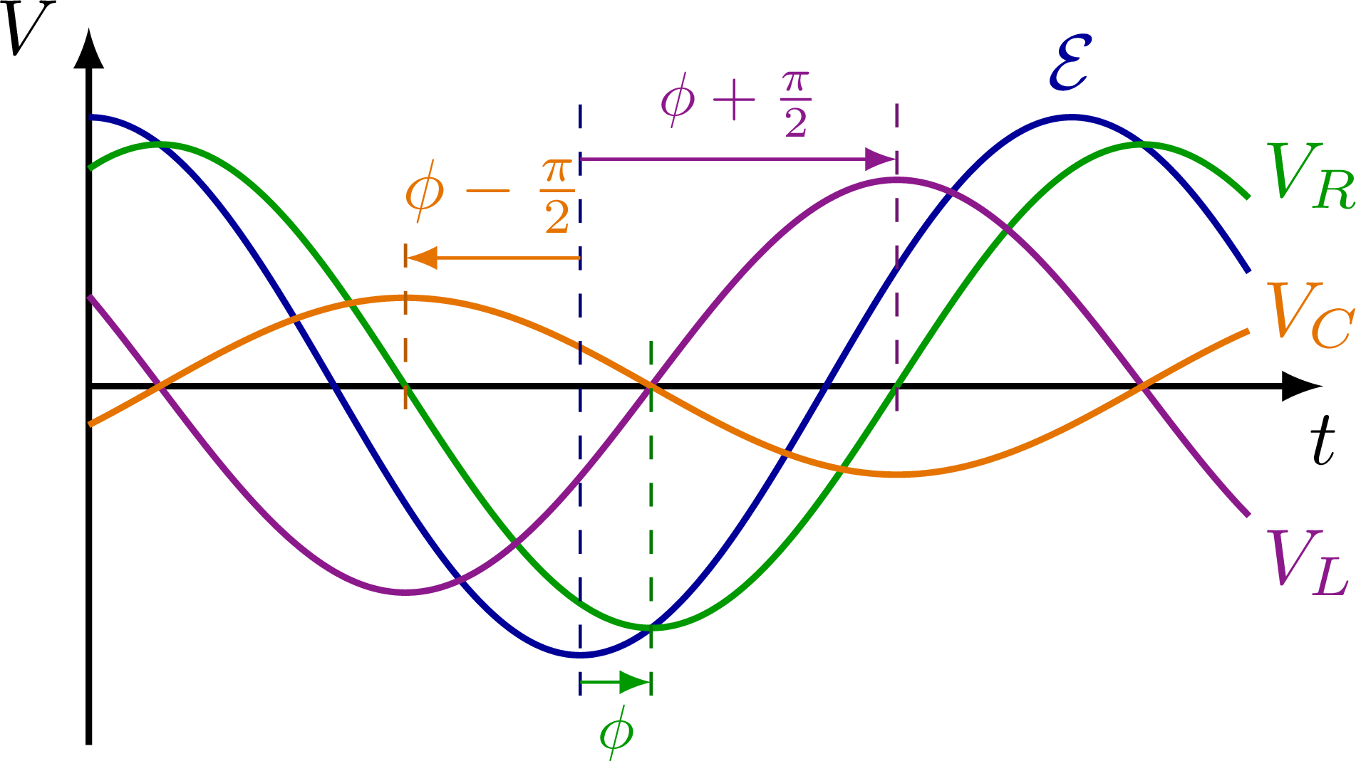
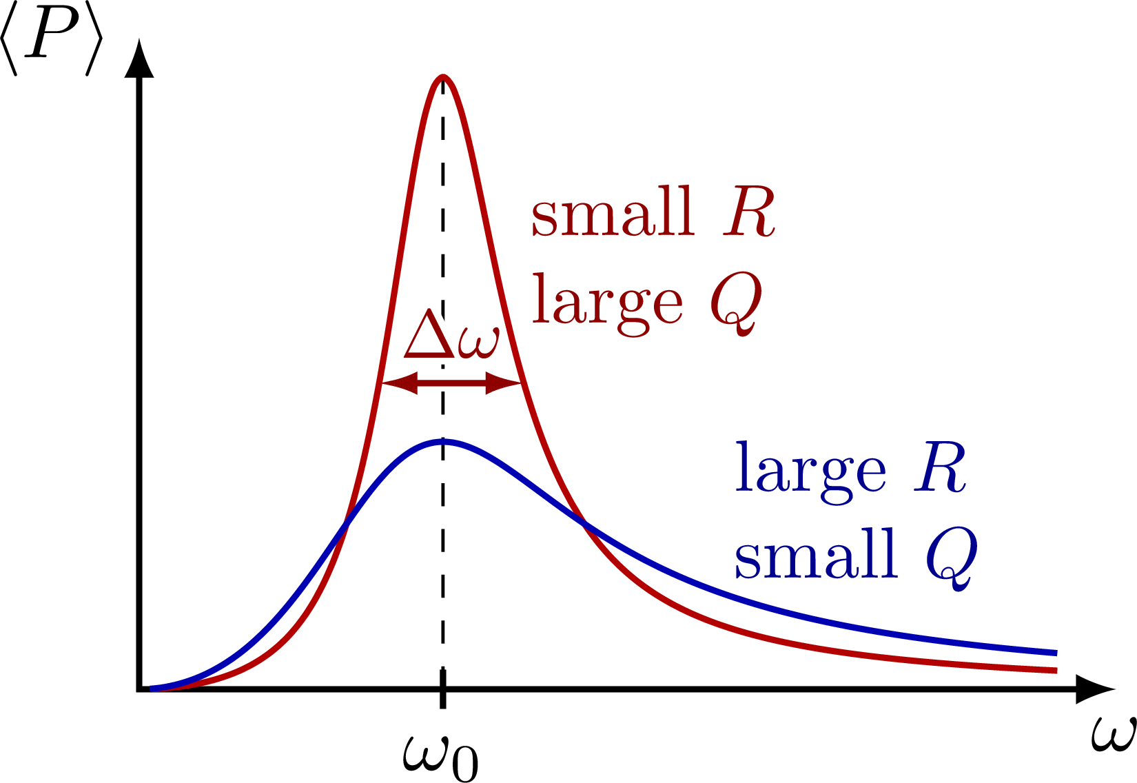
Plots of a circuit with alternating current and a resistor R, capacitor C and/or solenoid L, including an RLC circuit in series or in parallel. Also see the related circuit diagrams and phasors, or use the “circuits” tag.

Edit and compile if you like:

1
2
3
4
5
6
7
8
9
10
11
12
13
14
15
16
17
18
19
20
21
22
23
24
25
26
27
28
29
30
31
32
33
34
35
36
37
38
39
40
41
% Author: Izaak Neutelings (Februari, 2020)
\documentclass[border=3pt,tikz]{standalone}
\usepackage{amsmath} % for \dfrac
\usepackage{physics,siunitx}
\usepackage{tikz,pgfplots}
\usepackage[outline]{contour} % glow around text
\contourlength{1.0pt}
\usetikzlibrary{angles,quotes} % for pic (angle labels)
\usetikzlibrary{arrows.meta}
\usetikzlibrary{decorations.markings}
\tikzset{>=latex} % for LaTeX arrow head
\usepackage{xcolor}
\colorlet{Rcol}{green!60!black}
\colorlet{Ccol}{orange!90!black}
\colorlet{Lcol}{violet!90}
\colorlet{Icol}{blue!60!black}
\colorlet{myblue}{blue!70!black}
\colorlet{myred}{red!70!black}
\colorlet{Ecol}{orange!90!black}
\tikzstyle{Rline}=[Rcol,thick]
\tikzstyle{gline}=[Rcol,thick]
\tikzstyle{bline}=[myblue,thick]
\tikzstyle{rline}=[myred,thick]
\tikzstyle{width}=[{Latex[length=5,width=3]}-{Latex[length=5,width=3]},thick]
\def\xmax{5.5}
\def\ymax{1.6}
\def\A{1.2}
\def\I{1.1}
\def\om{(395/(0.94*\xmax))}
\def\tick#1#2{\draw[thick] (#1) ++ (#2:0.03*\ymax) --++ (#2-180:0.06*\ymax)}
\newcommand\EMF{\mathcal{E}} %\varepsilon}
\begin{document}
% AC circuit R
\begin{tikzpicture}
  \coordinate (O) at (0,0);
 
 
הההההההההההההההההההההההההההההההההההההההההההההההההההההההההההההההההההההההההההההההההההההההההההההההההההההההההההההההההההההההההההההההההההההההההההההההההההההההההההההההההההההההההההההההההההההההההההההההההההההההההההההההההההההההההההההההההההההההההההההההההההההההההההההההה
XXXXXXXXXXXXXXXXXXXXXXXXXXXXXXXXXXXXXXXXXXXXXXXXXXXXXXXXXXXXXXXXXXXXXXXXXXXXXXXXXXXXXXXXXXXXXXXXXXXXXXXXXXXXXXXXXXXXXXXXXXXXXXXXXXXXXXXXXXXXXXXXXXXXXXXXXXXXXXXXXXXXXXXXXXXXXXXXXXXXXXXXXXXXXXXXXXXXXXXXXXXXXXXXXXXXXXXXXXXXXXXXXXXXXXXXXXXXXXXXXXXXXXXXXXXXXXXX