")


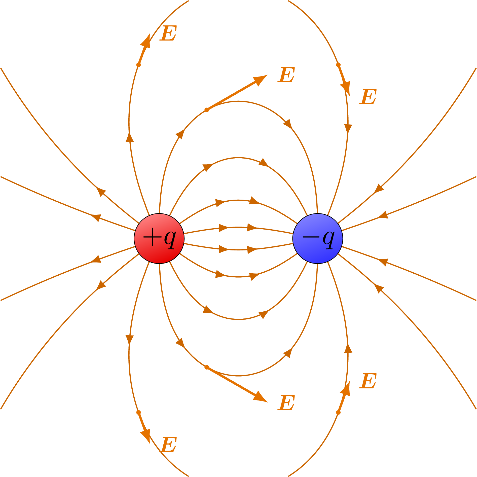
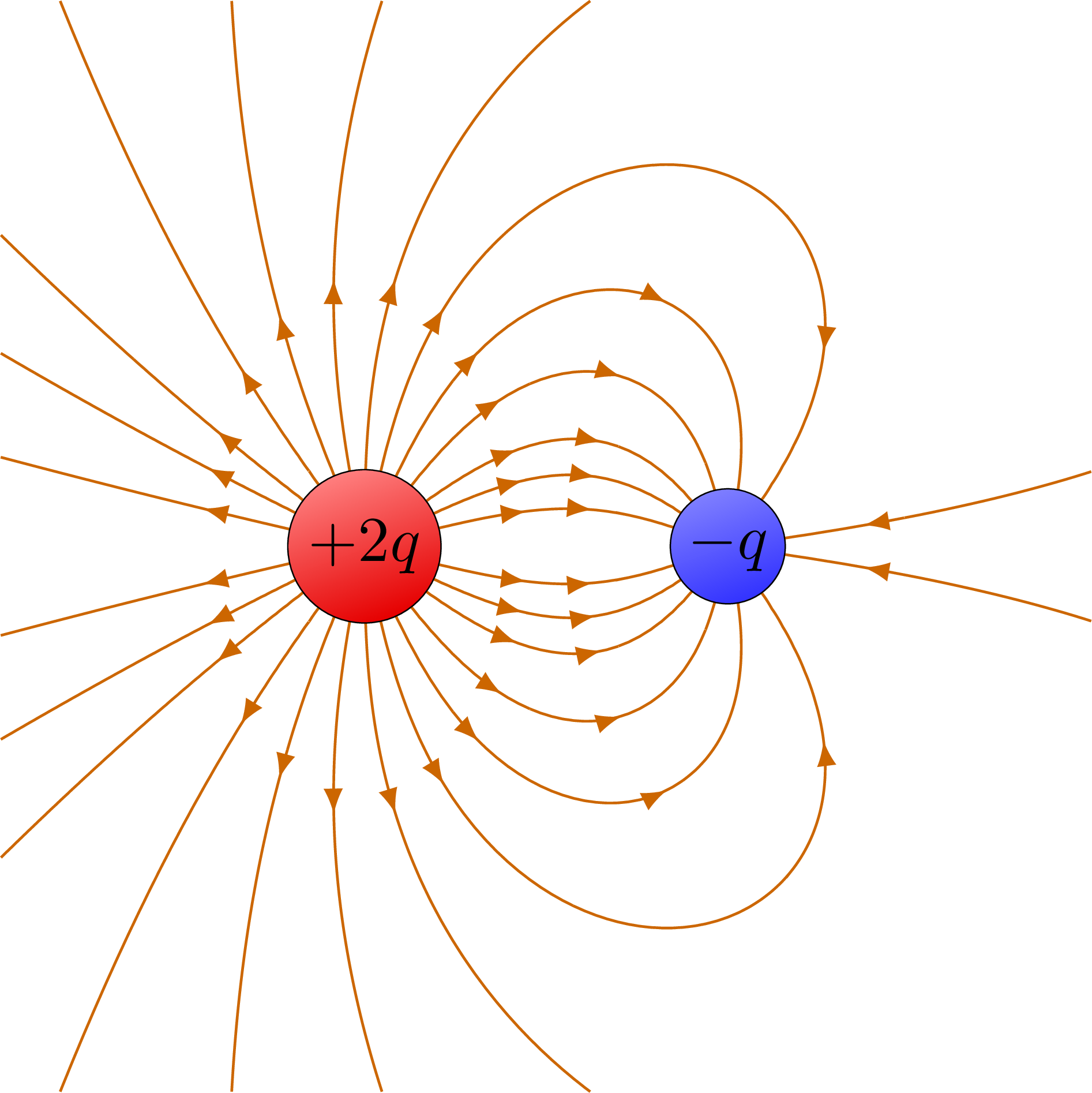
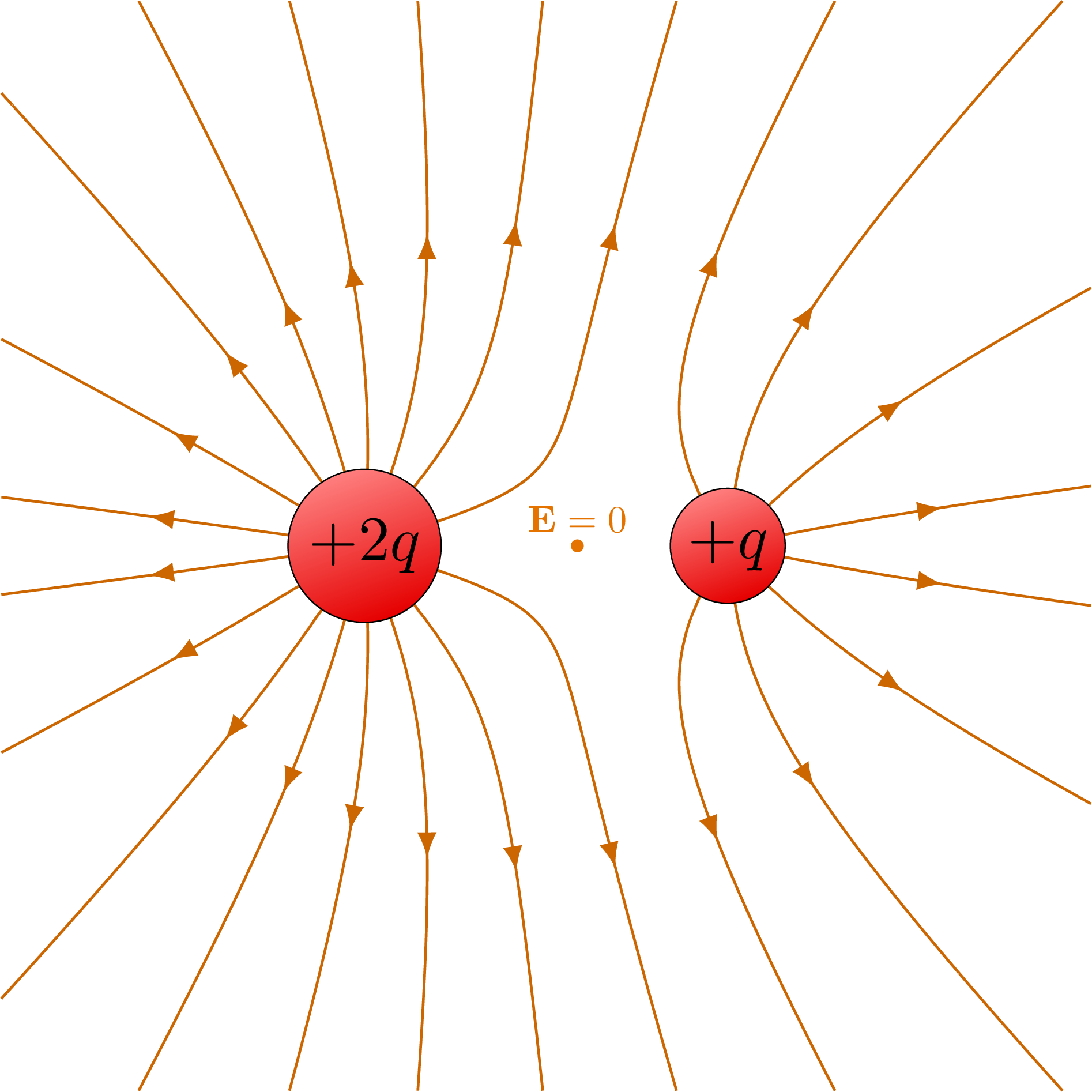
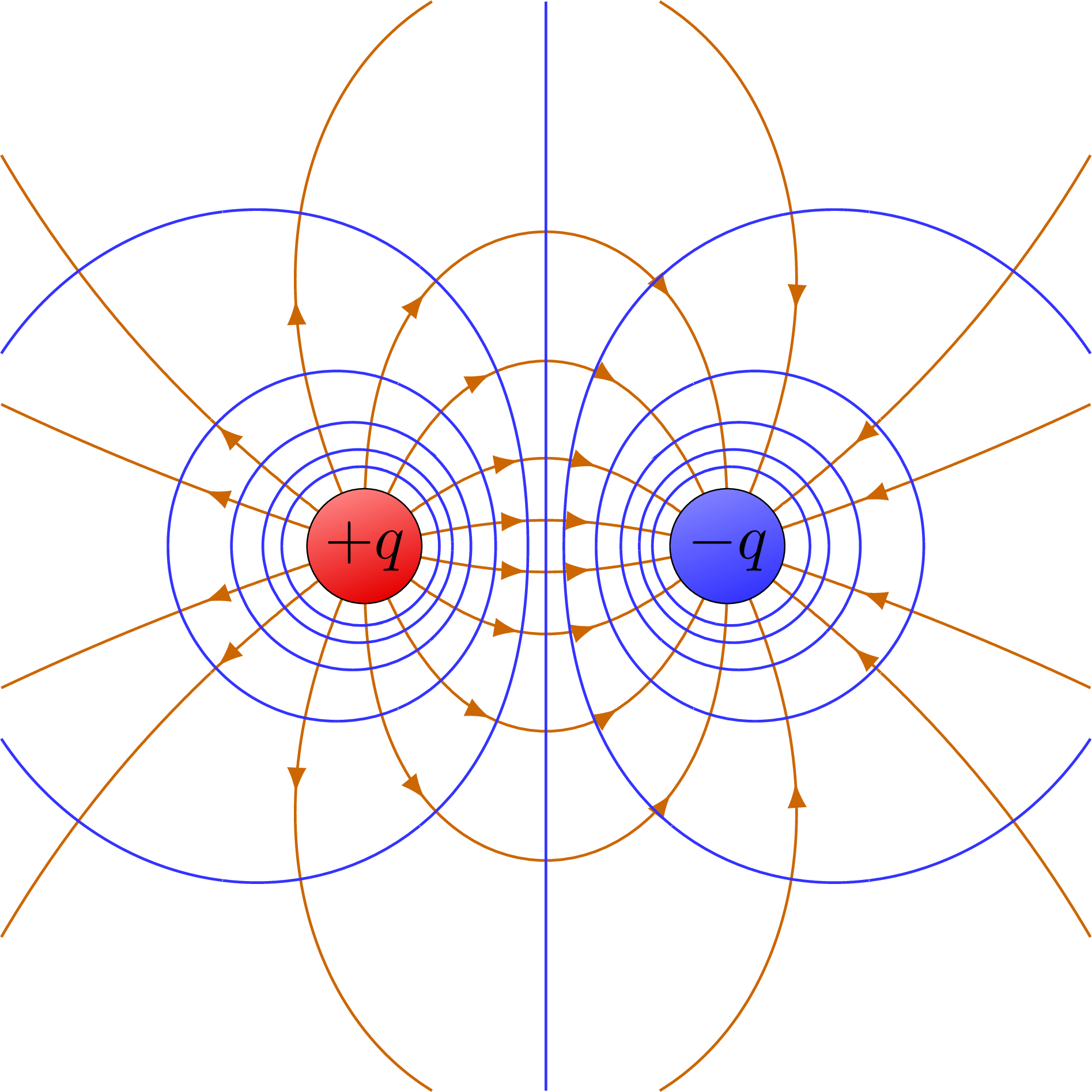
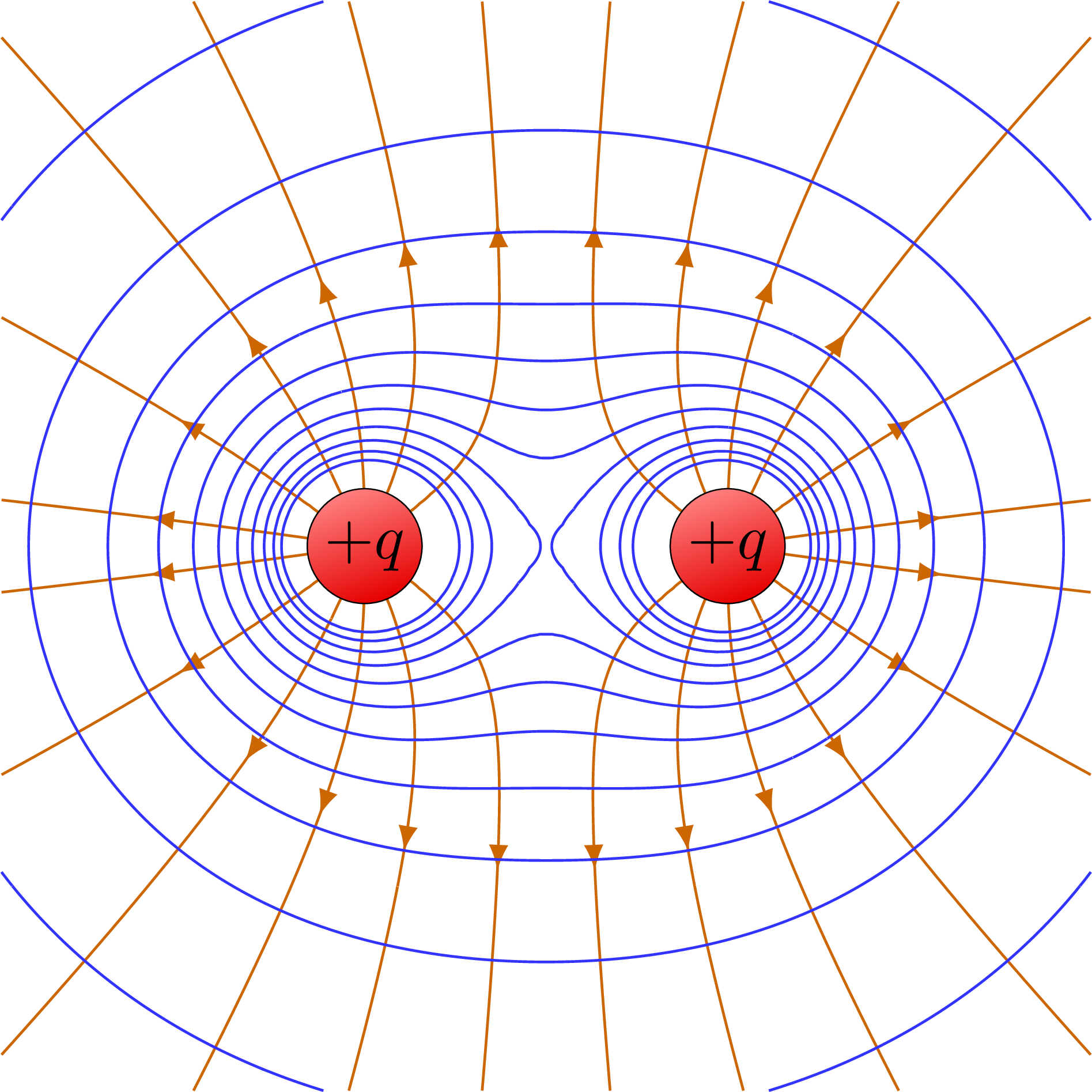
The electric field line and equipotential surfaces of two point charges: same-sign or opposite charge.

Download and compile the code below if you like, or try in Overleaf. Please note you may need to remove some tikzpicture pieces to avoid Overleaf’s time limit for compilation.
If you want to compile it on your own machine, make sure you have gnuplot installed, and you enable writing access to the LaTeX compiler by adding the command line option --enable-write18.
% Author: Izaak Neutelings (July 2018)
% page 8 https://archive.org/details/StaticAndDynamicElectricity
% https://stackoverflow.com/questions/4919827/gnuplot-with-texshop-in-osx --shell-escape
% https://tex.stackexchange.com/questions/56353/extract-x-y-coordinate-of-an-arbitrary-point-on-curve-in-tikz
% https://tex.stackexchange.com/questions/412899/tikz-calculate-and-store-the-euclidian-distance-between-two-coordinates

\documentclass[border=3pt,tikz]{standalone}
\usepackage{amsmath} % for \dfrac
\usepackage{bm}
\usepackage{tikz,pgfplots}
\tikzset{>=latex} % for LaTeX arrow head
\pgfplotsset{compat=1.13}
\usetikzlibrary{decorations.markings,intersections,calc}
\usepackage{ifthen}
%\usepackage{etoolbox}
\usepackage{xcolor}
\colorlet{Ecol}{orange!90!black}
\colorlet{EcolFL}{orange!80!black}
\colorlet{Bcol}{blue!90!black}
\tikzstyle{EcolEP}=[blue!80!white]
\tikzstyle{charge+}=[very thin,top color=red!50,bottom color=red!90!black,shading angle=20]
\tikzstyle{charge-}=[very thin,top color=blue!50,bottom color=blue!80,shading angle=20]
%\tikzstyle{EFielLineArrow2}=[
%    EcolFL,decoration={markings,
%          mark=at position 0.5 with {\arrow[rotate=\angle]{latex}}},
%          postaction={decorate}]
\tikzset{
   EFielLineArrow/.style args = {#1}{EcolFL,decoration={markings,
          mark=at position 0.5 with {\arrow[rotate=#1]{latex}}},
          postaction={decorate}}
}

\makeatletter
  \newcommand{\xy}[3]{% % FIND X, Y
    \tikz@scan@one@point\pgfutil@firstofone#1\relax
    \edef#2{\the\pgf@x}%
    \edef#3{\the\pgf@y}%
  }
\makeatother
\newcommand{\EFielLineArrow}[2]{ % ELECTRIC FIELD LINE ARROW
  \pgfkeys{/pgf/fpu,/pgf/fpu/output format=fixed} % for calculation between -1*10^324 and +1*10^324
  \pgfmathsetmacro{\x}{#1/28.45pt}
  \pgfmathsetmacro{\y}{#2/28.45pt}
  \pgfmathsetmacro{\U}{\Q*((\x+\a)^2+(\y)^2)^(3/2)}
  \pgfmathsetmacro{\V}{\q*((\x-\a)^2+(\y)^2)^(3/2)}
  \pgfkeys{/pgf/fpu=false}
  \pgfmathparse{
    atan2(((\y)*\V + (\y)*\U),((\x+\a)*\V + (\x-\a)*\U))
  }
  \edef\angle{\pgfmathresult}
  \pgfmathsetmacro{\D}{int(1000*\q*(\x+\a)/sqrt((\x+\a)^2+\y*\y) + 1000*\Q*(\x-\a)/sqrt((\x-\a)^2+\y*\y))/1000}
  \draw[EFielLineArrow={\angle}] (\xpt,\ypt);
}
\newcommand{\EVector}[2]{ % ELECTRIC FIELD VECTOR
  \pgfmathsetmacro{\x}{#1/28.45pt}
  \pgfmathsetmacro{\y}{#2/28.45pt}
  \pgfmathsetmacro{\U}{((\x+\a)^2+(\y)^2)^(3/2)}
  \pgfmathsetmacro{\V}{((\x-\a)^2+(\y)^2)^(3/2)}
  \pgfmathsetmacro{\Ex}{\q*3*(\x+\a)/\U + \Q*3*(\x-\a)/\V}
  \pgfmathsetmacro{\Ey}{\q*3*(\y)/\U + \Q*3*(\y)/\V}
  \fill[Ecol] (\x,\y) circle (0.8pt);
  \draw[->,Ecol,thick] (\x,\y) --++ (\Ex,\Ey)
    node[Ecol,right,scale=0.8] {$\bm{E}$};
  \pgfmathsetmacro{\D}{int(1000*\q*(\x+\a)/sqrt((\x+\a)^2+\y*\y) + 1000*\Q*(\x-\a)/sqrt((\x-\a)^2+\y*\y))/1000}
}
\newcommand{\EFieldLines}{ % ELECTRIC FIELD LINES
  \message{^^JField lines (\q,\Q) with contours range ^^J\range^^J}

  % PATHS for intersections
  \path[name path=ellipse1] (-\a,0) ellipse ({0.90*\R} and {1.5*\R});
  \path[name path=ellipse2] (+\a,0) ellipse ({0.75*\R} and {1.5*\R});
  \path[name path=ellipse3] (  0,0) ellipse ({\a+\R} and 1.5*\R);

  % FIELD LINES
  \draw[EcolFL,name path=Elines] plot[id=plot, raw gnuplot, smooth]
    function{
       f(x,y) = \q*(x+\a)/sqrt((x+\a)**2+y**2) + \Q*(x-\a)/sqrt((x-\a)**2+y**2);
       set xrange [\xmin:\xmax];
       set yrange [-\ymax:\ymax];
       set view 0,0;
       set isosample 400,400;
       set cont base;
       set cntrparam levels discrete \range;
       unset surface;
       splot f(x,y)
    };

  % ELLIPSE INTERSECTIONS
  \pgfmathsetmacro{\oppositesign}{\q*\Q<0 ? 1 : 0}
  \ifthenelse{\oppositesign>0}{
    % OPPOSITE SIGN
    \foreach \c in {1,2}{
      \message{Intersections \c...}
      \path[name intersections={of=Elines and ellipse\c,total=\t}]
        \pgfextra{\xdef\Nb{\t}};
      \message{ found \Nb ^^J}
      \foreach \i in {1,...,\Nb}{
        \message{  \i}
        \xy{(intersection-\i)}{\xpt}{\ypt}
        \EFielLineArrow{\xpt}{\ypt}
        \message{ (\D,\x,\y)^^J}
      }
    }
  }{
    % SAME SIGN
    \message{Intersections...}
    \path[name intersections={of=Elines and ellipse3,total=\t}]
        \pgfextra{\xdef\Nb{\t}};
    \message{ found \Nb ^^J}
    \foreach \i in {1,...,\Nb}{
      \message{  \i}
      \xy{(intersection-\i)}{\xpt}{\ypt}
      \EFielLineArrow{\xpt}{\ypt}
      \message{ (\D,\x,\y)^^J}
    }
  }
}
\newcommand{\EEquipot}{ % EQUIPOTENTIAL SURFACE
  \message{^^JEquipotential surface (\q,\Q) with contours range ^^J\rangeEP}

  % FIELD LINES
  \draw[EcolEP] plot[id=plot, raw gnuplot, smooth] %,dashed
    function{
       f(x,y) = \q/sqrt((x+\a)**2+y**2) + \Q/sqrt((x-\a)**2+y**2);
       set xrange [\xmin:\xmax];
       set yrange [-\ymax:\ymax];
       set view 0,0;
       set isosample 400,400;
       set cont base;
       set cntrparam levels discrete \rangeEP;
       unset surface;
       splot f(x,y)
    };
}
\newcommand{\EVectorOnFieldLines}{ % ELECTRIC FIELD VECTOR
  \message{^^JVector on field lines (\q,\Q) with contours range ^^J\C^^J}

  % FIELD LINES
  \path[name path=xline] (\Cx,-\ymax) -- (\Cx,-\a) (\Cx,\a) -- (\Cx,\ymax);
  \path[name path=Elines] plot[id=plot, raw gnuplot, smooth]
    function{
       f(x,y) = \q*(x+\a)/sqrt((x+\a)**2+y**2) + \Q*(x-\a)/sqrt((x-\a)**2+y**2);
       set xrange [\xmin:\xmax];
       set yrange [-\ymax:\ymax];
       set view 0,0;
       set isosample 100,100;
       set cont base;
       set cntrparam levels discrete \C;
       unset surface;
       splot f(x,y)
    };

    \message{Intersections...}
    \path[name intersections={of=Elines and xline,total=\t}]
      \pgfextra{\xdef\Nb{\t}};
    \message{ found \Nb ^^J}
    \foreach \i in {1,...,\Nb}{
      \message{  \i}
      \xy{(intersection-\i)}{\xpt}{\ypt}
      \EVector{\xpt}{\ypt}
      \message{ (\D,\x,\y)^^J}
    }
}


\begin{document}


% OPPOSITE, +1 -1
\begin{tikzpicture}
  \def\xmin{-3}
  \def\xmax{3}
  \def\ymax{3}
  \def\a{1}
  \def\q{+1}
  \def\Q{-1}
  \def\R{1.0}
  \def\range{0.05,0.2,0.6,1.0,1.4,1.8,1.98}

  % LINES
  \EFieldLines

  % VECTORS
  \def\Cx{-0.4}
  \def\C{0.6,1.0}
  \EVectorOnFieldLines
  \def\Cx{-1.26}
  \EVectorOnFieldLines
  \def\Cx{1.26}
  \EVectorOnFieldLines

  % CHARGES
  \draw[charge+] (-\a,0) circle (9pt) node[black,scale=1.0] {$+q$};
  \draw[charge-] (+\a,0) circle (9pt) node[black,scale=1.0] {$-q$};

\end{tikzpicture}


%% OPPOSITE, +2 -1
%\begin{tikzpicture}
%  \def\xmin{-3}
%  \def\xmax{3}
%  \def\ymax{3}
%  \def\a{1}
%  \def\q{+2}
%  \def\Q{-1}
%  \def\R{1.0}
%  %\def\range{-2.9,-2.8,-2.6,-2.2,-1.8,-1.4,
%  %           -1.01,-0.6,-0.2,0.2,0.6,0.8,1.0,1.2}
%  \def\range{-0.95,-0.8,-0.6,-0.2,0.2,0.6,
%             1.01,1.4,1.8,2.2,2.6,2.8,2.94}
%
%  % LINES
%  \EFieldLines
%
%  % CHARGES
%  \draw[charge+] (-\a,0) circle (12pt) node[black,scale=1.0] {$+2q$};
%  \draw[charge-] (+\a,0) circle ( 9pt) node[black,scale=1.0] {$-q$};
%
%\end{tikzpicture}


%% OPPOSITE, +1 +1
%\begin{tikzpicture}
%  \def\xmin{-3}
%  \def\xmax{3}
%  \def\ymax{3}
%  \def\a{1}
%  \def\q{+1}
%  \def\Q{+1}
%  \def\R{1.2}
%  \def\range{-1.99,-1.8,-1.4,-1.0,-0.6,-0.2,
%             0.2,0.6,1.0,1.4,1.8,1.99}
%
%  % LINES
%  \EFieldLines
%
%  % VECTORS
%  \def\Cx{-1.42}
%  \def\C{-1.0}
%  \EVectorOnFieldLines
%  \def\Cx{-0.85}
%  \def\C{-0.6}
%  \EVectorOnFieldLines
%  \fill[Ecol] (0,0) circle (1pt) node[Ecol,above,scale=0.7] {$\mathbf{E}=0$};
%
%  % CHARGES
%  \draw[charge+] (-\a,0) circle (9pt) node[black,scale=1.0] {$+q$};
%  \draw[charge+] (+\a,0) circle (9pt) node[black,scale=1.0] {$+q$};
%
%\end{tikzpicture}


%% OPPOSITE, +2 +1 (equipotential surface)
%\begin{tikzpicture}
%  \def\xmin{-3}
%  \def\xmax{3}
%  \def\ymax{3}
%  \def\a{1}
%  \def\q{+2}
%  \def\Q{+1}
%  \def\R{1.2}
%  \def\range{-2.98,-2.7,-2.1,-1.5,-0.9,-0.3,
%              0.3,0.9,1.5,2.1,2.7,2.98}
%
%  % LINES
%  \EFieldLines
%  \fill[Ecol] ({(3-2*sqrt(2))*\a},0) circle (1pt) node[Ecol,above,scale=0.6] {$\mathbf{E}=0$};
%
%  % CHARGES
%  \draw[charge+] (-\a,0) circle (12pt) node[black,scale=1.0] {$+2q$};
%  \draw[charge+] (+\a,0) circle ( 9pt) node[black,scale=1.0] {$+q$};
%
%\end{tikzpicture}


%% OPPOSITE, +1 -1 (equipotential surface)
%\begin{tikzpicture}
%  \def\xmin{-3}
%  \def\xmax{3}
%  \def\ymax{3}
%  \def\a{1}
%  \def\q{+1}
%  \def\Q{-1}
%  \def\R{1.0}
%  \def\range{0.05,0.2,0.6,1.0,1.4,1.8,1.98}
%  \def\rangeEP{-1.8,-1.4,-1.0,-0.6,-0.2,0.0,0.2,0.6,1.0,1.4,1.8}
%
%  % LINES
%  \EFieldLines
%  \EEquipot
%
%  % CHARGES
%  \draw[charge+] (-\a,0) circle (9pt) node[black,scale=1.0] {$+q$};
%  \draw[charge-] (+\a,0) circle (9pt) node[black,scale=1.0] {$-q$};
%
%\end{tikzpicture}


%% OPPOSITE, +1 +1 (equipotential surface)
%\begin{tikzpicture}
%  \def\xmin{-3}
%  \def\xmax{3}
%  \def\ymax{3}
%  \def\a{1}
%  \def\q{+1}
%  \def\Q{+1}
%  \def\R{1.2}
%  \def\range{-1.99,-1.8,-1.4,-1.0,-0.6,-0.2,
%             0.2,0.6,1.0,1.4,1.8,1.99}
%  \def\rangeEP{0.0,0.1,0.2,0.4,0.6,0.8,1.0,1.2,1.4,1.6,1.8,2.002,2.2,2.4,2.6}
%  %-1.8,-1.4,-1.0,-0.6,-0.2,
%
%  % LINES
%  \EFieldLines
%  \EEquipot
%
%  % CHARGES
%  \draw[charge+] (-\a,0) circle (9pt) node[black,scale=1.0] {$+q$};
%  \draw[charge+] (+\a,0) circle (9pt) node[black,scale=1.0] {$+q$};
%
%\end{tikzpicture}


\end{document}
Click to download: electric_fieldlines2.tex • electric_fieldlines2.pdf
Open in Overleaf: electric_fieldlines2.tex


")


Hi
What a great job on you website !
There is an issue with this particular template of electric field lines of two charges. Works neither on the web page, nor with overleaf, nor locally.
Is it possible to get the correct template ?
many thanks
Hi Ronan,
Apologies for the late reply, I only saw this comment now.
I could run the full template locally without problem, but it can take up to 4 min. because the code looks for intersections between the field lines and an ellipse to place the arrows. (Granted, not the most efficient method.)
Overleaf did not finish the compilation of the full code because it took too long, but if you simply comment out or remove most of the tikzpictures, it should compile the remaining ones within the time limit.
Compiling on this tikz.net page sady does not work, because gnuplot need to create new files for the field lines, and I think web users do not have writing access to the servers for security reasons.
Hope that helps!
Izaak
Hi Izaak
I tried with Texstudio but it did not work due to an issue of no shape name “intersection-1” is known.
Thank you for your consideration.
Best regards,
Hey Duc,
Sorry for the late reply!
Did you perhaps run the code after changing something like the contour ranges in \range or the figure size? To place arrowheads on the field lines, the \EFieldLines macro computes intersections with an ellipse or straight line. I guess no intersections were found (\Nb=0), so the foreach “\foreach \i in {1,…,\Nb}” tries to loop from 1 to 0, but “intersection-1” and “intersection-0” do not exist. This might require some finetuning of the contours or ellipse, or you could just remove this snippet in \EFieldLines.
Cheers,
Izaak
Hi Izaak,
I want to continue on this thread regarding the error. I am running your code locally on my machine, and I am getting the same error as Duc. Everywhere where you called the commands – \EFieldLines, \EVectorOnFieldLines, \EVectorOnFieldLines and \EVectorOnFieldLines, I get the error –
Package pgf Warning: Plot data file `TestLatex.plot.table’ not found. on input line 182.
Intersections 1… found 0
1
! Package pgf Error: No shape named intersection-1 is known.
See the pgf package documentation for explanation.
Type H for immediate help.
…
l.182 \EFieldLines
This error message was generated by an \errmessage
command, so I can’t give any explicit help.
Pretend that you’re Hercule Poirot: Examine all clues,
and deduce the truth by order and method.
(2.0,0.0,0.0)
0
! Package pgf Error: No shape named intersection-0 is known.
See the pgf package documentation for explanation.
Type H for immediate help.
…
I hope this detailed error log helps you in fixing the error. Please look at this issue.
-Ani
Hey Ani, thank you for the error message. You can see it says
Package pgf Warning: Plot data file `TestLatex.plot.table’ not found.
which means something went probably wrong in this line:
  \draw[EcolFL,name path=Elines] plot[id=plot, raw gnuplot, smooth]

    function{

       % ...

    };
and the extra
*.plot.tablefile was not created.Can you check that you have gnuplot installed, please?
http://www.gnuplot.info/download.html
On Linux or macOS, you can check in a terminal with for example
which gnuplot
If you have it installed, you may also need to give the LaTeX compiler writing access via
--enable-write18to create the*.plot.tablefile.Hope that helps,
Izaak
Hi Izaak,
Thank you for a fast reply. That means a lot!
I went over your instructions and found that gnuplot is installed in my MAC. I also checked my editor and found that –shell-escape is enabled (I think –shell-escape is same as –enable-write18. Correct me if I am wrong.) With –shell-escape, it did not work and it gave me the same error.
Thanks,
-Ani
Hi Ani,
No problem!
Can you make sure that gnuplot is in the search path for the LaTeX compiler? For example, on my Mac, this shell command
dirname `which gnuplot`tells me it’s in/usr/local/bin/. Maybe your gnuplot is in a weird location, so the compiler cannot find it? If you are using some editor like TeXShop, you could try adding this directory to the search path in preferences, or create a symlink.If that does not work, can you check with
--enable-write18anyway, please?Other than those two things, I am not sure what would solve the problem for you…
Cheers,
Izaak
Hi Izaak,
Thank you so much for the help. I have been able to resolve this issue. I guess I should explain the solution for other users here –
1. I am explaining the steps here for a MAC user. For windows users, I will try to explain as much as possible.
2. You need gnuplot to be installed for this code to work. In windows you can easily install it from the sourceforge link (https://sourceforge.net/projects/gnuplot/files/gnuplot/5.4.4/). For MAC the best way to install it is using homebrew. First install homebrew if you have not installed it before (https://brew.sh/). Once that is installed, download and install gnuplot from homebrew (https://formulae.brew.sh/formula/gnuplot).
3. Homebrew automatically downloads and installs the gnuplot on MAC. It also adds necessary paths in the MAC for other programs to find it when required. By default the path is /opt/homebrew/bin/gnuplot. However, none of the Latex editors can find it from that path where homebrew instals it. So create a sym link in MAC by using this command “- sudo ln -s /opt/homebrew/bin/gnuplot /usr/local/bin/gnuplot”. It will ask for your password.
4. In windows make sure that the installer for gnuplot adds its path in the environment variable of windows. If not manually add the location in the environment variables location (google how to add paths in windows).
4. Once that is done, compile your latex file using the “-shell-escape” mode.
5. The entire code takes close to 5 to 8 mins to run. Just wait and it will compile fine.
Great! Thanks for the explanation! Glad we could solve this.
Hi
How can I export png or svg for these ?
`pdflatex –shell-escape`
Works but it gave me pdf which I want png or SVG and sadly I am new to tikz and latex I am learning.
Hi Korosh,
To convert to PNG, I typically use an external tool like Preview on macOS or ImageMagick‘s command line tool. If it’s installed on your system, you can run something like the following, to convert the first page of a multipage PDF to a PNG:
convert -density 1500 -trim electric_fieldlines2.pdf[0] Efield-001.png
Although, the command is renamed to
magicknow:magick -density 1500 -trim electric_fieldlines2.pdf[0] Efield-001.png
For SVG, you have to Google yourself, I am afraid. There are StackExchange threads like this one.
What do you need SVG for? Generally, for vector quality, I would suggest sticking to PDF. If you need a single-page file, you could simply split the TEX file into one per
tikzpicture.Cheers,
Izaak
Thanks Izaak
I needed SVG because I made an Application with web tech like Electron, which translates SVG with Node. I needed SVG vectors for both quality and scaling reasons.
I found tex2svg and found your StackExchange thread useful.
For the png part, I had to install ImageMagick, which I couldn’t do with brew because my macOS is High Sierra 10.13.6 (outdated). Then I found MacPort can install it, but again, I found out MacPort and HomeBrew can’t coexist together on non-ARM MacBooks. For older devices like mine, you can install both, but when you want to compile, remove the other one from PATH, like I installed ImageMagick with MacPort and removed brew from PATH during compiling.
Just in case anyone else has the same issues as me.
I recommend MacPort on older devices.
Install Macport on older macOS and brew for newer macOS, then install ImageMagick (which will install dozens of packages to compile on your macOS) > tex.
The path for MacPort is: /opt/local.
The path for Brew (non-ARM) is: /usr/local
.