Linear Approximation 3d

Edit and compile if you like:

\documentclass{article}
\usepackage{tikz}
\usepackage{tikz-3dplot}
\usetikzlibrary{math}
\usepackage{ifthen}
\usepackage[active,tightpage]{preview}
\PreviewEnvironment{tikzpicture}
\setlength\PreviewBorder{1pt}
%
% File name: linear-approximation-3d.tex
% Description: 
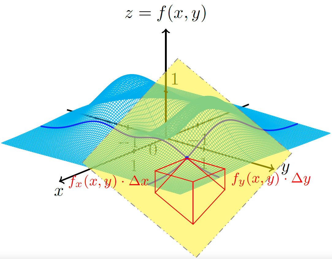
% The linear approximation for a function of two variables $z = f(x,y)$ is shown.
% 
% Date of creation: March, 7th, 2021.
% Date of last modification: October, 9th, 2022.
% Author: Efraín Soto Apolinar.
% https://www.aprendematematicas.org.mx/author/efrain-soto-apolinar/instructing-courses/
% Source: page 15 of the 
% Glosario Ilustrado de Matem\'aticas Escolares.
% https://tinyurl.com/5udm2ufy
%
% Terms of use:
% According to TikZ.net
% https://creativecommons.org/licenses/by-nc-sa/4.0/
% Your commitment to the terms of use is greatly appreciated.
%
\begin{document}
%
\tdplotsetmaincoords{70}{130}
%
\begin{tikzpicture}[tdplot_main_coords]
	% functions
	\tikzmath{function funcion(\x,\y) {return (\x*\x+3*\y*\y)*e^(-\x*\x-\y*\y);};} % the function $z = f(x,y)$
	\tikzmath{function derivadax(\x,\y) {return -2.0*\x*(-1.0 + \x * \x + 3.0 * \y * \y) * exp(-\x*\x - \y*\y);};}	% $f_{x}$
	\tikzmath{function derivaday(\x,\y) {return -2.0*\y*(-3.0 + \x * \x + 3.0 * \y * \y) * exp(-\x*\x - \y*\y);};}	% $f_{y}$
	% equation of the plane
	\tikzmath{function plano(\x,\y) {return derivadax(\xcero,\ycero)*(\x-\xcero)+derivaday(\xcero,\ycero)*(\y-\ycero)+\zcero;};}
	%	
	\pgfmathsetmacro{\dominio}{0.75*pi}	% domain for plotting
	\pgfmathsetmacro{\step}{\dominio/50.0} % step size
	\pgfmathsetmacro{\max}{\dominio}
	\pgfmathsetmacro{\xi}{-\dominio}
	\pgfmathsetmacro{\xf}{\dominio}
	\pgfmathsetmacro{\xe}{\xf+\step}
	\pgfmathsetmacro{\xs}{\xi+\step}
	\pgfmathsetmacro{\yi}{-\dominio}
	\pgfmathsetmacro{\yf}{\dominio}
	\pgfmathsetmacro{\ys}{\yi+\step}
	\pgfmathsetmacro{\ye}{\yf+\step}
	\pgfmathsetmacro{\h}{1}
	%  size of the tangent plane
	\pgfmathsetmacro{\size}{1.5}
	% Point of tangency $(\x_{0}, y_{0}, z_{0})$
	\pgfmathsetmacro{\xcero}{1.125} 
	\pgfmathsetmacro{\ycero}{1.5} 
	\pgfmathsetmacro{\zcero}{funcion(\xcero,\ycero)}
	\pgfmathsetmacro{\dx}{1.0}
	\pgfmathsetmacro{\dy}{1.0}
	\pgfmathsetmacro{\zplanoxi}{plano(\xcero,\ycero)}
	\pgfmathsetmacro{\zplanoxf}{plano(\xcero+\dx,\ycero)}
	\pgfmathsetmacro{\zplanoyi}{plano(\xcero,\ycero)}
	\pgfmathsetmacro{\zplanoyf}{plano(\xcero,\ycero+\dx)}
	\pgfmathsetmacro{\zplanoxyf}{plano(\xcero+\dx,\ycero+\dx)}
	% Region where the tangent plane is shown
	\pgfmathsetmacro{\Ax}{\xcero-\size}
	\pgfmathsetmacro{\Ay}{\ycero-\size}
	\pgfmathsetmacro{\Bx}{\xcero+\size}
	\pgfmathsetmacro{\By}{\ycero-\size}
	\pgfmathsetmacro{\Cx}{\xcero+\size}
	\pgfmathsetmacro{\Cy}{\ycero+\size}
	\pgfmathsetmacro{\Dx}{\xcero-\size}
	\pgfmathsetmacro{\Dy}{\ycero+\size}
	% Vertices of the tangent plane
	\pgfmathsetmacro{\Az}{plano(\Ax,\Ay)}
	\pgfmathsetmacro{\Bz}{plano(\Bx,\By)}
	\pgfmathsetmacro{\Cz}{plano(\Cx,\Cy)}
	\pgfmathsetmacro{\Dz}{plano(\Dx,\Dy)}
	%
	\pgfmathsetmacro{\zmax}{funcion(-\max,-\max)}
	\pgfmathsetmacro{\zorigen}{funcion(0,0)}
	\pgfmathsetmacro{\zplano}{plano(0,0)}
	% Plot the graph in the third and second quadrants 
	% The graph of $z = f(x,y)$: third quadrant
	\foreach \x in {\xi,\xs,...,0}{
		\draw[cyan,opacity=0.75] plot[domain=\yi:0,smooth,variable=\t] ({\x},{\t},{funcion(\x,\t)});
	}
	\foreach \y in {\yi,\ys,...,0}{
		\draw[cyan,opacity=0.75] plot[domain=\yi:0,smooth,variable=\t] ({\t},{\y},{funcion(\t,\y)});
	}
	% negative part of the coordinate axis
	\draw[thick] (\xi-0.25,0,0) -- (0,0,0); % x axis
	\draw[thick] (0,\yi-0.25,0,0) -- (0,0,0); % y axis
	\foreach \x in {-1,1}
		\draw[thick] (\x,0,0.05) -- (\x,0,-0.05) node [below] {$\x$};
	\foreach \y in {-1,1}
		\draw[thick] (0,\y,0.05) -- (0,\y,-0.05) node [below] {$\y$};
	\foreach \z/\posicion in {0/below left}
		\draw[thick] (0,0.05,\z) -- (0,-0.05,\z) node [\posicion] {$\z$};
	% The graph of $z = f(x,y)$: second quadrant
	\foreach \x in {\xi,\xs,...,0}{
		\draw[cyan,opacity=0.75] plot[domain=0:\yf,smooth,variable=\t] ({\x},{\t},{funcion(\x,\t)});
	}
	\foreach \y in {0,\step,...,\yf}{
		\draw[cyan,opacity=0.75] plot[domain=\xi:0,smooth,variable=\t] ({\t},{\y},{funcion(\t,\y)});
	}
	% The graph of $z = f(x,y)$: fouth quadrant
	\foreach \x in {0,\step,...,\xf}{
		\draw[cyan,opacity=0.75] plot[domain=\yi:0,smooth,variable=\t] ({\x},{\t},{funcion(\x,\t)});
	}
	\foreach \y in {\yi,\ys,...,0}{
		\draw[cyan,opacity=0.75] plot[domain=0:\yf,smooth,variable=\t] ({\t},{\y},{funcion(\t,\y)});
	}	
	% coordinate axis
	\draw[thick] (0,0,0) -- (0,\yf+0.5,0); % Eje y
	\draw[thick,->] (0,0,0) -- (\xf+1.0,0,0) node [below] {$x$};
	\draw[thick,->] (0,\yf,0) -- (0,\yf+0.5,0) node [right] {$y$};
	\draw[thick] (0,0,0) -- (0,0,\zplano,0);
	\foreach \z/\posicion in {1/above right}
		\draw[thick] (0,0.05,\z) -- (0,-0.05,\z) node [\posicion] {$\z$};
	% The graph of $z = f(x,y)$: first quadrant
	\foreach \x in {0,\step,...,\xf}{
		\draw[cyan,opacity=0.75] plot[domain=0:\yf,smooth,variable=\t] ({\x},{\t},{funcion(\x,\t)});
	}
	\foreach \y in {0,\step,...,\yf}{
		\draw[cyan,opacity=0.75] plot[domain=0:\yf,smooth,variable=\t] ({\t},{\y},{funcion(\t,\y)});
	}	
	% plot of $z = f(x,y)$ for $y$ constant
	\draw[blue,thick] plot[domain=-\dominio:\dominio,smooth,variable=\t,samples=100] ({\t},{\ycero},{funcion(\t,\ycero)});
	% plot of $z = f(x,y)$ for $x$ constant
	\draw[blue,thick] plot[domain=-\dominio:\dominio,smooth,variable=\t,samples=100] ({\xcero},{\t},{funcion(\xcero,\t)});
	% the edge of the plane
	\fill[yellow,opacity=0.5] (\Ax,\Ay,\Az) -- (\Bx,\By,\Bz) -- (\Cx,\Cy,\Cz) -- (\Dx,\Dy,\Dz) -- (\Ax,\Ay,\Az);
	\draw[gray,dash dot dot] (\Ax,\Ay,\Az) -- (\Bx,\By,\Bz) -- (\Cx,\Cy,\Cz) -- (\Dx,\Dy,\Dz) -- (\Ax,\Ay,\Az);
	% The point of tangency
	\fill[blue] (\xcero,\ycero,\zcero) circle (1pt);		
	% Last part of the $z$ axis
	\draw[thick,->] (0,0,\zplano) -- (0,0,\max) node[above] {$z = f(x,y)$}; 
	% Increment $\Delta x$
	\draw[red,thin] (\xcero,\ycero,\zcero) 
		-- (\xcero+\dx,\ycero,\zcero) 
		-- (\xcero+\dx,\ycero,\zplanoxf) node[left,midway] {\footnotesize$f_{x}(x,y)\cdot \Delta x$}
		-- (\xcero,\ycero,\zcero);
	% Increment $\Delta y$
	\draw[red,thin] (\xcero,\ycero,\zcero) 
		-- (\xcero,\ycero+\dy,\zcero) 
		-- (\xcero,\ycero+\dy,\zplanoyf) node[right,midway] {\footnotesize$f_{y}(x,y)\cdot \Delta y$}
		-- (\xcero,\ycero,\zcero);
	% Total increment for $z$
	\draw[red,thin] (\xcero,\ycero,\zcero) -- (\xcero+\dx,\ycero,\zcero) -- (\xcero+\dx,\ycero+\dy,\zcero) -- (\xcero,\ycero+\dy,\zcero) -- (\xcero,\ycero,\zcero);
	\draw[red,thin] (\xcero+\dx,\ycero,\zplanoxf) -- (\xcero+\dx, \ycero+\dy, \zplanoxyf) -- (\xcero,\ycero+\dy,\zplanoyf);
	\draw[red,thin] (\xcero+\dx, \ycero+\dy, \zplanoxyf) -- (\xcero+\dx, \ycero+\dy, \zcero);
\end{tikzpicture}
%
\end{document}