Malus Law

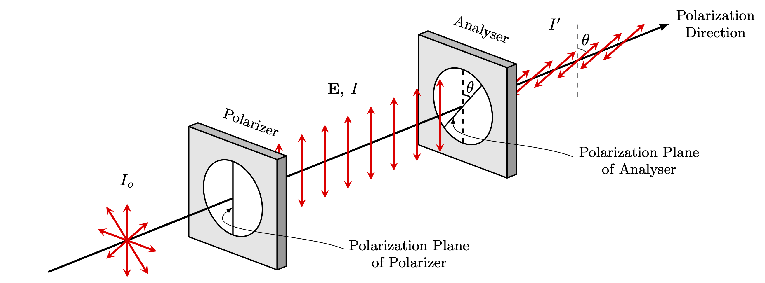
Edit and compile if you like:

\documentclass[border=3pt]{standalone}

% Drawing
\usepackage{tikz}

% Tikz Library
\usetikzlibrary{3d, shapes.multipart, angles, quotes}

% Tikz Styles
\tikzset{>=latex}
\tikzset{axis/.style={black, very thick, ->}}
\tikzset{ef/.style={very thick, red}}
\tikzset{vec/.style={black, -{Latex[length=0.8mm]}}}
\tikzset{every text node part/.style={align=center}}

% Newcommand
%% Polar Coordinates Line from (0,0 to (r, theta)
\newcommand{\cdraw}[2]{\draw[very thick, -stealth, red] (0,0) -- ({#1*cos(#2)}, {#1*sin(#2)});}
%% Polarizer
\newcommand{\polarizer}[2]{%
	\begin{scope}[canvas is xz plane at y=1.2]
		\draw[line join=round, thick, fill=black!40] (#1,-1.2) rectangle (#1+0.2,1.2);
	\end{scope}
	%
	\begin{scope}[canvas is xy plane at z=1.2]
		\draw[line join=round, thick, fill=black!25](#1,-1.2) rectangle (#1+0.2,1.2);
	\end{scope}
	%
	\begin{scope}[canvas is yz plane at x=#1]
		\draw[line join=round, thick, fill=black!10] (-1.2,-1.2) rectangle (1.2,1.2);
		\draw[line join=round, thick, fill=white] (0,0) circle (0.8cm);
		\draw[line join=round, thick] (-{0.8*cos(#2)}, -{0.8*sin(#2)}) -- ({0.8*cos(#2)},{0.8*sin(#2)});
	\end{scope}
}
%% Analyser
\newcommand{\analizer}[2]{%
	\begin{scope}[canvas is xz plane at y=1.2]
		\draw[line join=round, thick, fill=black!40] (#1,-1.2) rectangle (#1+0.2,1.2);
	\end{scope}
	%
	\begin{scope}[canvas is xy plane at z=1.2]
		\draw[line join=round, thick, fill=black!25](#1,-1.2) rectangle (#1+0.2,1.2);
	\end{scope}
	%
	\begin{scope}[canvas is yz plane at x=#1]
		\draw[line join=round, thick, fill=black!10] (-1.2,-1.2) rectangle (1.2,1.2);
		\draw[line join=round, thick, fill=white] (0,0) coordinate (B) circle (0.8cm);
		\draw[line join=round, thick] (-{0.8*cos(#2)}, -{0.8*sin(#2)}) -- ({0.8*cos(#2)},{0.8*sin(#2)}) coordinate (A);
		\draw[line join=round, dashed, thick] (0,-0.8) -- (0,0.8) coordinate (C);
		\pic[line join=round, draw, thick, "$\theta$", angle radius=0.25cm, angle eccentricity=1.8] {angle = A--B--C};
	\end{scope}
}

% Notation
\usepackage{amsmath}

\begin{document}

%Layers
\pgfdeclarelayer{layer1}
\pgfdeclarelayer{layer2}
\pgfdeclarelayer{layer3}
\pgfdeclarelayer{layer4}
\pgfdeclarelayer{layer5}
\pgfdeclarelayer{layer6}
\pgfdeclarelayer{layer7}

\pgfsetlayers{main, layer7, layer6, layer5, layer4, layer3, layer2, layer1}

\begin{tikzpicture}[x={(1cm,0.4cm)}, y={(8mm, -3mm)}, z={(0cm,1cm)}, line cap=round, line join=round]
	
	% Main Axes
%	\draw[->] (0,0,0) -- (12,0,0) node[right] {$x$};
%	\draw[->] (0,0,0) -- (0,2,0) node[below left] {$y$};
%	\draw[->] (0,0,0) -- (0,0,2) node[above] {$z$};
	
	% Big Axis 
	\draw[axis] (-1,0,0) -- (12.5,0,0) node[right, black] {\small{Polarization}\\[-0.5mm]\small{Direction}};
	
	% Polarizers
	\begin{pgfonlayer}{layer1}
		\polarizer{3}{90}
	\end{pgfonlayer}
	\begin{pgfonlayer}{layer3}
		\analizer{8}{50}
	\end{pgfonlayer}
	
	% Polarizer and Analiyzer Nodes
	\begin{scope}[canvas is yz plane at x=3]
		\node[rotate=-20] at (0.5,1.8) {\small{Polarizer}};
	\end{scope}
	%
	\begin{scope}[canvas is yz plane at x=8]
		\node[rotate=-20] at (0.5,1.8) {\small{Analyser}};
	\end{scope}
	
	% Polarization Planes
	\begin{pgfonlayer}{layer1}
		\begin{scope}[canvas is xy plane at z=-0.2]
			\draw[latex-] (3,0) to[out=160, in=270] (3,3) node[right, yshift=-3pt] {\small{Polarization Plane}\\[-0.5mm]\small{of Polarizer}};
		\end{scope}
		%
		\begin{scope}[canvas is xy plane at z=-0.2]
			\draw[latex-] (7.85,-0.07) to[out=130, in=270] (8,3) node[right, yshift=-3pt] {\small{Polarization Plane}\\[-0.5mm]\small{of Analyser}};
		\end{scope}
	\end{pgfonlayer}
	
	% Electric Field
	%% Physical Light
	\begin{pgfonlayer}{layer1}
		\begin{scope}[canvas is yz plane at x=0.7]
			\foreach \i in {0,45,...,315}
			{
				\cdraw{0.8}{\i}
			}		
		\end{scope}		
	\end{pgfonlayer}
	
	%% Linear Polarization
	\begin{pgfonlayer}{layer2}
		\begin{scope}[canvas is yz plane at x=5.4]
			\node at (0,1.4) {$\mathbf E, \: I$};
		\end{scope}
		\foreach \i in {3,3.5,...,7.5}
		{
			\begin{scope}[canvas is yz plane at x=\i]
				\cdraw{0.8}{90}
				\cdraw{0.8}{270}
			\end{scope}
		}
	\end{pgfonlayer}
	
	%% Slanted Linear Polarization
	\begin{pgfonlayer}{layer4}
		\begin{scope}[canvas is yz plane at x=10.5]
			\draw[dashed] (0,-0.8) -- (0,0.8);
			\coordinate (A) at ({0.8*cos(45)},{0.8*sin(45)});
			\coordinate (B) at (0,0);
			\coordinate (C) at (0,0.8); 
			\pic[draw,  "$\theta$", angle radius=0.25cm, angle eccentricity=2, pic text options={xshift=-1pt}] {angle = A--B--C};
		\end{scope}
		\foreach \i in {8,8.5,...,11.5}
		{
			\begin{scope}[canvas is yz plane at x=\i]
				\cdraw{0.8}{45}
				\cdraw{0.8}{225}
			\end{scope}
	
		}		
	\end{pgfonlayer}
	
	% Nodes
	\node at (0.7,0,1.3) {$I_o$};
	\node at (10,0,1) {$I'$};
	
	% Refinements for 3D View
	\begin{pgfonlayer}{layer1}
		\draw[very thick] (1,0,0) -- (2.99,0,0);
	\end{pgfonlayer}
	\begin{pgfonlayer}{layer3}
		\draw[very thick] (6,0,0) -- (7.99,0,0);
	\end{pgfonlayer}
\end{tikzpicture}

\end{document}