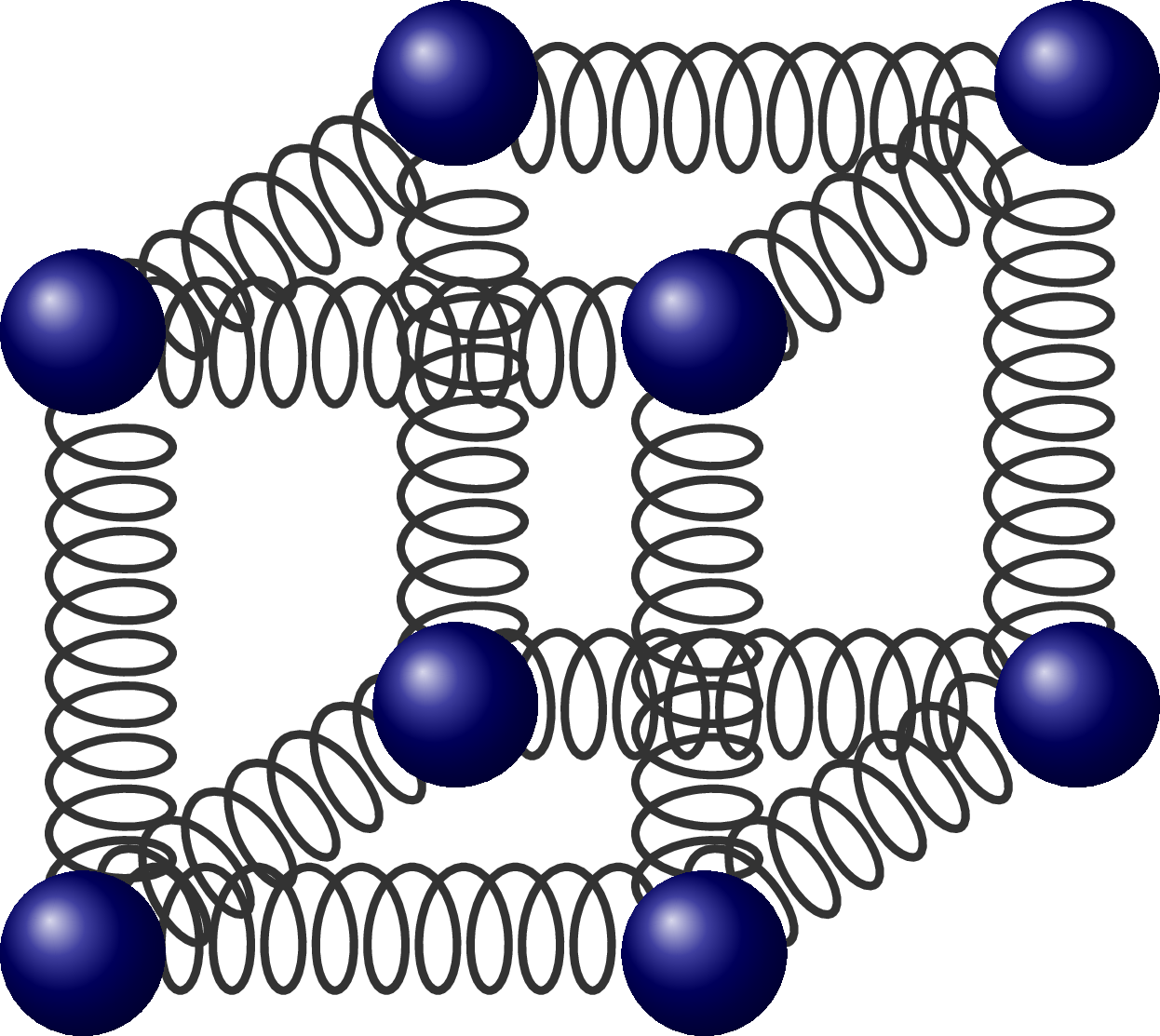
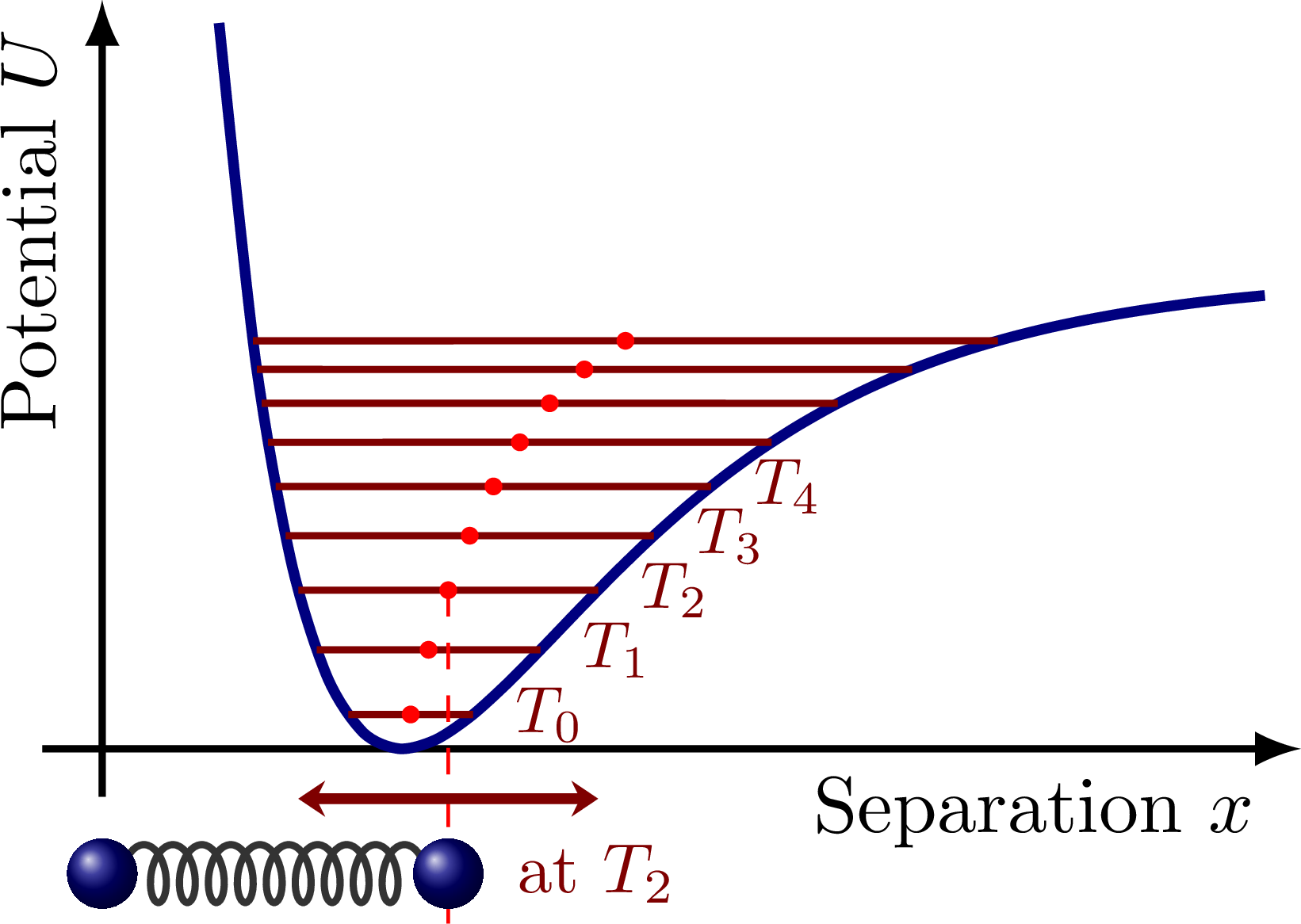
Molecular vibrations

Molecular vibration illustrated with springs, and the Morse potential with different energy levels. Also see these diagrams on harmonic oscillator approximations.

Edit and compile if you like:

1
2
3
4
5
6
7
8
9
10
11
12
13
14
15
16
17
18
19
20
21
22
23
24
25
26
27
28
29
30
31
32
33
34
35
36
37
38
39
40
41
% Author: Izaak Neutelings (March 2019)
\documentclass[border=3pt,tikz]{standalone}
\usepackage{tikz}
\usepackage{ifthen}
\tikzset{>=latex} % for LaTeX arrow head
\usetikzlibrary{calc} 
\usetikzlibrary{patterns,snakes,decorations.pathmorphing,intersections,arrows.meta}
\begin{document}
\tikzstyle{atom}=[ball color=blue!50!black]
\tikzstyle{bound}=[thick,black!80,decorate,decoration={coil,amplitude=6pt,segment length=5pt}]
% BOUNDS
\begin{tikzpicture}[scale=2,z={(0.6,0.4)}]
  \def\z{-.03}
  \def\o{1.03}
  
  \draw[bound] (0,0,0) -- (1,0,0);
  \draw[bound] (0,0,0) -- (0,1,0);
  \draw[bound] (0,0,0) -- (0,0,1);
  \draw[bound] (1,0,0) -- (1,1,0);
  \draw[bound] (1,0,0) -- (1,0,1);
  \draw[bound] (0,1,0) -- (1,1,0);
  \draw[bound] (0,1,0) -- (0,1,1);
  \draw[bound] (0,0,1) -- (0,1,1);
  \draw[bound] (0,0,1) -- (1,0,1);
  \draw[bound] (1,1,0) -- (1,1,1);
  \draw[bound] (0,1,1) -- (1,1,1);
  \draw[bound] (1,0,1) -- (1,1,1);
  \fill[atom] (\z,\z,\z) circle (4pt);
  \fill[atom] (\o,\z,\z) circle (4pt);
  \fill[atom] (\z,\o,\z) circle (4pt);
  \fill[atom] (\z,\z,\o) circle (4pt);
  \fill[atom] (\o,\o,\z) circle (4pt);
  \fill[atom] (\o,\z,\o) circle (4pt);
  \fill[atom] (\z,\o,\o) circle (4pt);
  \fill[atom] (\o,\o,\o) circle (4pt);
  
\end{tikzpicture}
 
 
הההההההההההההההההההההההההההההההההההההההההההההההההההההההההההההההההההההההההההההההההההההההההההההההההההההההההההההההההההההההההההההההההההההההההההההההההההההההההההההההההההההההההההההההההההההההההההההההההההההההההההההההההההההההההההההההההההההההההההההההההההההההההההההההה
XXXXXXXXXXXXXXXXXXXXXXXXXXXXXXXXXXXXXXXXXXXXXXXXXXXXXXXXXXXXXXXXXXXXXXXXXXXXXXXXXXXXXXXXXXXXXXXXXXXXXXXXXXXXXXXXXXXXXXXXXXXXXXXXXXXXXXXXXXXXXXXXXXXXXXXXXXXXXXXXXXXXXXXXXXXXXXXXXXXXXXXXXXXXXXXXXXXXXXXXXXXXXXXXXXXXXXXXXXXXXXXXXXXXXXXXXXXXXXXXXXXXXXXXXXXXXXXX