Harmonic oscillator approximation

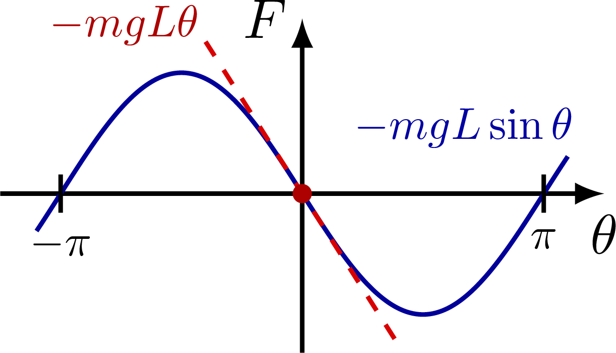
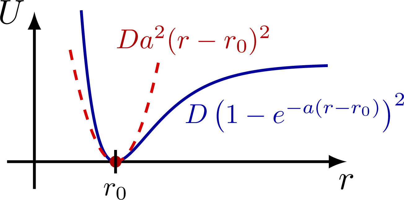
Taylor expansion of the potential energy of a pendulum and molecule, in order to approximate it with a simple harmonic oscillator. Also see the these plots of the general solutions, these phase portraits, and pendulum diagrams.
These figures are used in Ben Kilminster’s lecture notes for PHY111.

Approximate the gravitational force on a pendulum with a Hooke’s law, which is equivalent to the small-angle approximation:

Approximate the potential energy of a pendulum with a parabola to get a simple harmonic oscillator:

Approximate the potential energy of the force between atoms in a diatomic molecule (Morse potential) with a parabola:

Edit and compile if you like:

% Author: Izaak Neutelings (Februari 2021)
\documentclass[border=3pt,tikz]{standalone}
\usepackage{amsmath} % for \dfrac
\usepackage{physics,siunitx}
\usepackage{tikz,pgfplots}
\usepackage[outline]{contour} % glow around text
\contourlength{1.0pt}
\usetikzlibrary{angles,quotes} % for pic (angle labels)
\usetikzlibrary{arrows.meta}
\usetikzlibrary{decorations.markings}
\tikzset{>=latex} % for LaTeX arrow head
\usepackage{xcolor}

\colorlet{xcol}{blue!60!black}
\colorlet{myred}{red!85!black}
\colorlet{myblue}{blue!80!black}
\colorlet{mycyan}{cyan!80!black}
\colorlet{mygreen}{green!70!black}
\colorlet{myorange}{orange!90!black!80}
\colorlet{mypurple}{red!50!blue!90!black!80}
\colorlet{mydarkred}{myred!80!black}
\colorlet{mydarkblue}{myblue!80!black}
\tikzstyle{xline}=[xcol,thick]
\tikzstyle{Tline}=[line width=0.6]
\tikzstyle{width}=[{Latex[length=5,width=3]}-{Latex[length=5,width=3]},thick]
\def\tick#1#2{\draw[thick] (#1)++(#2:0.12) --++ (#2-180:0.24)}
\def\N{100} % number of samples


\begin{document}


% HARMONIC OSCILLATOR FORCE
\begin{tikzpicture}
  \message{^^JHarmonic oscillation}
  \def\ymax{1.0}  % max y axis
  \def\xmax{1.9}  % max x axis
  \def\A{0.76}        % amplitude
  \def\T{(1.6*\xmax)} % period
  \draw[->,thick] (0,-\ymax) -- (0,1.1*\ymax) node[left=-1] {$F$};
  \draw[->,thick] (-\xmax,0) -- (\xmax,0) node[below] {$\theta$};
  \draw[xline,samples=100+\N,smooth,variable=\x,domain=-0.88*\xmax:0.88*\xmax]
    plot(\x,{-\A*sin(360/\T*\x)});
  \draw[xline,myred,dashed,samples=\N,smooth,variable=\x,domain=-0.20*\T:0.20*\T] %,line cap=round
    plot(\x,{-\A*2*pi/\T*\x});
  \fill[myred!80!black] (0,0) circle(0.06);
  \tick{{-\T/2},0}{90} node[below=0,scale=0.8] {$-\pi$};
  \tick{{ \T/2},0}{90} node[below=0,scale=0.8] {$\pi$};
  \node[mydarkblue,above left=0,scale=0.8] at (0.95*\xmax,0.25*\A) {$-mgL\sin\theta$};
  \node[mydarkred,above left=0,scale=0.8] at (-0.29*\xmax,1.1*\A) {$-mgL\theta$};
\end{tikzpicture}


% HARMONIC OSCILLATOR ENERGY
\def\ymax{1.4} % max y axis
\begin{tikzpicture}
  \def\xmax{2.6} % max x axis
  \message{^^JHarmonic oscillation}
  \def\A{0.6}         % amplitude
  \def\T{(0.7*\xmax)} % period
  \draw[->,thick] (0,-0.2*\ymax) -- (0,1.1*\ymax) node[left=-1] {$U$};
  \draw[->,thick] (-\xmax,0) -- (\xmax,0) node[below] {$\theta$};
  \draw[xline,samples=100+\N,smooth,variable=\x,domain=-0.94*\xmax:0.94*\xmax]
    plot(\x,{\A-\A*cos(360/\T*\x)});
  \draw[xline,myred,dashed,samples=\N,smooth,variable=\x,domain={-0.33*\T}:{0.34*\T}]
    plot(\x,{\A/2*(2*pi*\x/\T)^2});
  \fill[myred!80!black] (0,0) circle(0.06);
  \tick{{\T},0}{90} node[below=0,scale=0.8] {$2\pi$};
  \tick{{-\T},0}{90} node[below=0,scale=0.8] {$-2\pi$};
  \node[mydarkred,above left,scale=0.8] at ({-0.28*\T},2.05*\A) {$\frac{mgL}{2}\theta^2$};
  \node[mydarkblue,above right,scale=0.8] at ({0.43*\T},1.95*\A) {$mgL(1-\cos\theta)$}; %U(\theta)=
\end{tikzpicture}


% MORSE POTENTIAL
\begin{tikzpicture}
  \message{^^JMorse potential}
  \def\xmax{3.2} % max x axis
  \def\A{1}
  \def\b{2.3}
  \def\a{(0.26*\xmax)}
  \draw[->,thick] (0,-0.2*\ymax) -- (0,1.1*\ymax) node[left=-1] {$U$};
  \draw[->,thick] (-0.2*\ymax,0) -- (\xmax,0) node[below] {$r$};
  \draw[xline,samples=100+\N,smooth,variable=\x,domain=0.15*\xmax:0.94*\xmax]
    plot(\x,{\A*(1-exp(-\b*(\x-\a)))^2});
  \draw[xline,myred,dashed,samples=\N,smooth,variable=\x,domain=0.44*\a:1.55*\a] %,line cap=round
    plot(\x,{\A*\b^2*(\x-\a)^2});
  \fill[myred!80!black] ({\a},0) circle(0.06);
  \tick{{\a},0}{90} node[below=0,scale=0.8] {$r_0$};
  \node[mydarkblue,above right,scale=0.8] at (0.45*\xmax,0.2*\A) {$D\left(1-e^{-a(r-r_0)}\right)^2$};
  \node[mydarkred,scale=0.8] at (0.51*\xmax,0.89*\ymax) {$Da^2(r-r_0)^2$};
\end{tikzpicture}


\end{document}