")


Some plots of the general solutions of simple, damped, and drive harmonic oscillator. Also see these Taylor approximations, and phase portraits.
These figures are used in Ben Kilminster’s lecture notes for PHY111.
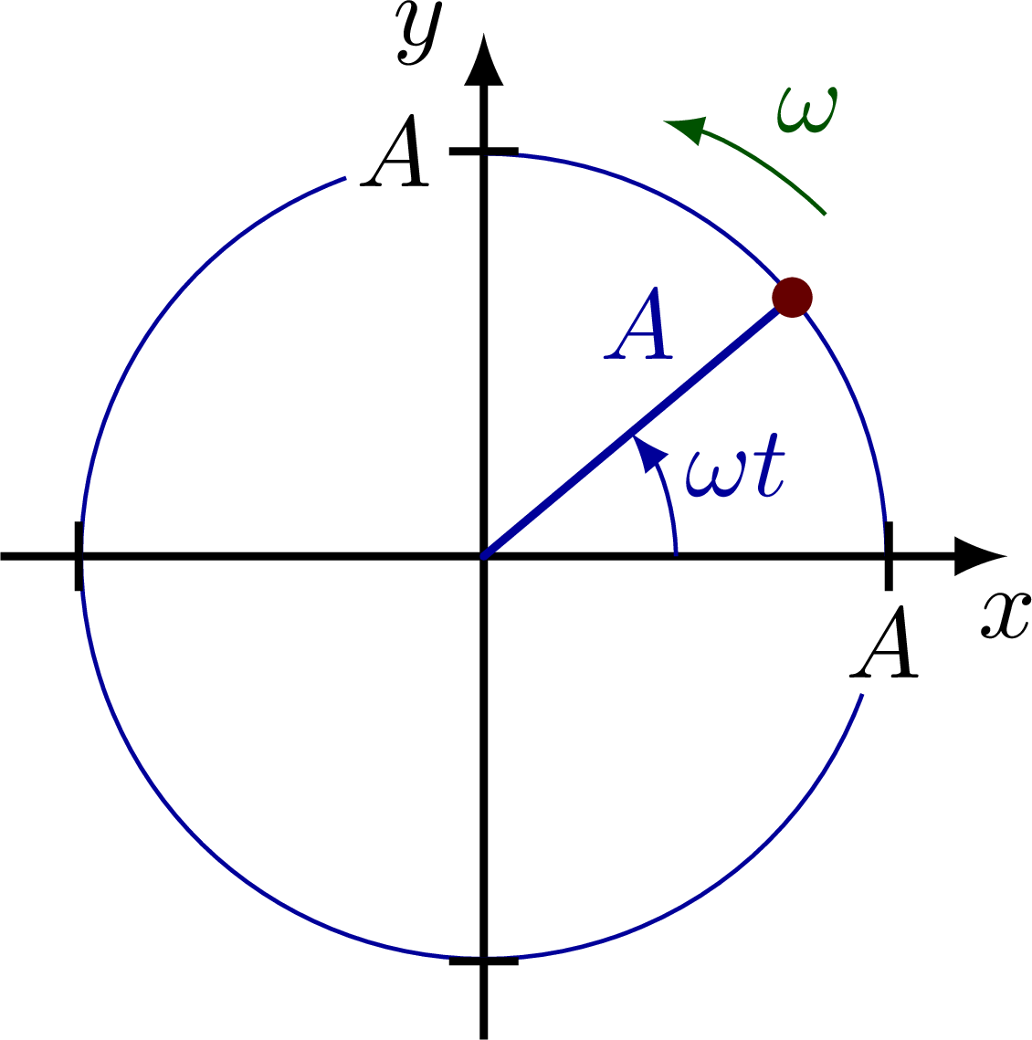
Simple harmonic oscillator as a uniformly rotating point on a circle (a “phasor”), where the projection onto the x axis gives a cosine wave.
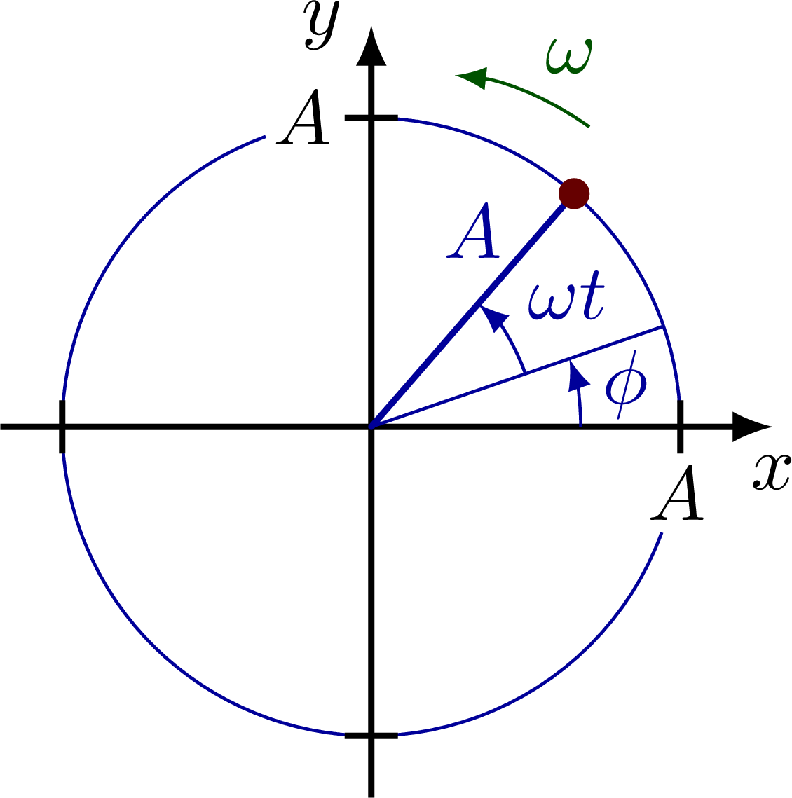
Simple harmonic oscillator on a circle with a phase shift φ.
Simple harmonic oscillator as a cosine wave: displacement versus time with the period T indicate.

Simple harmonic oscillator as a sine wave with a phase shift.

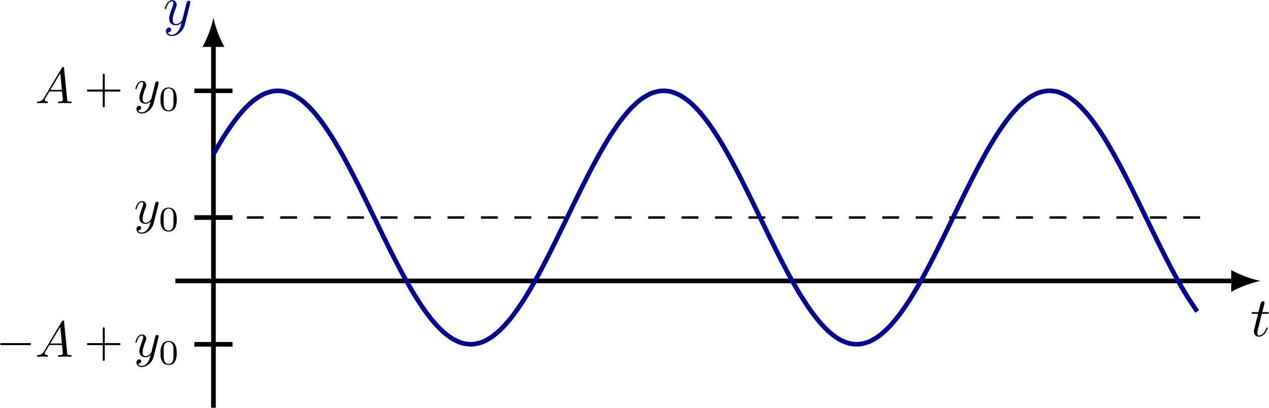
Simple harmonic oscillator with a displaced rest position (e.g. for a vertical spring):
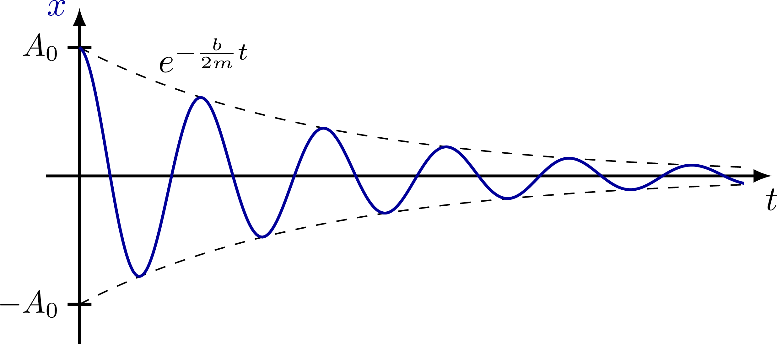
Damped harmonic oscillator with a exponential decay factor as an envelop.
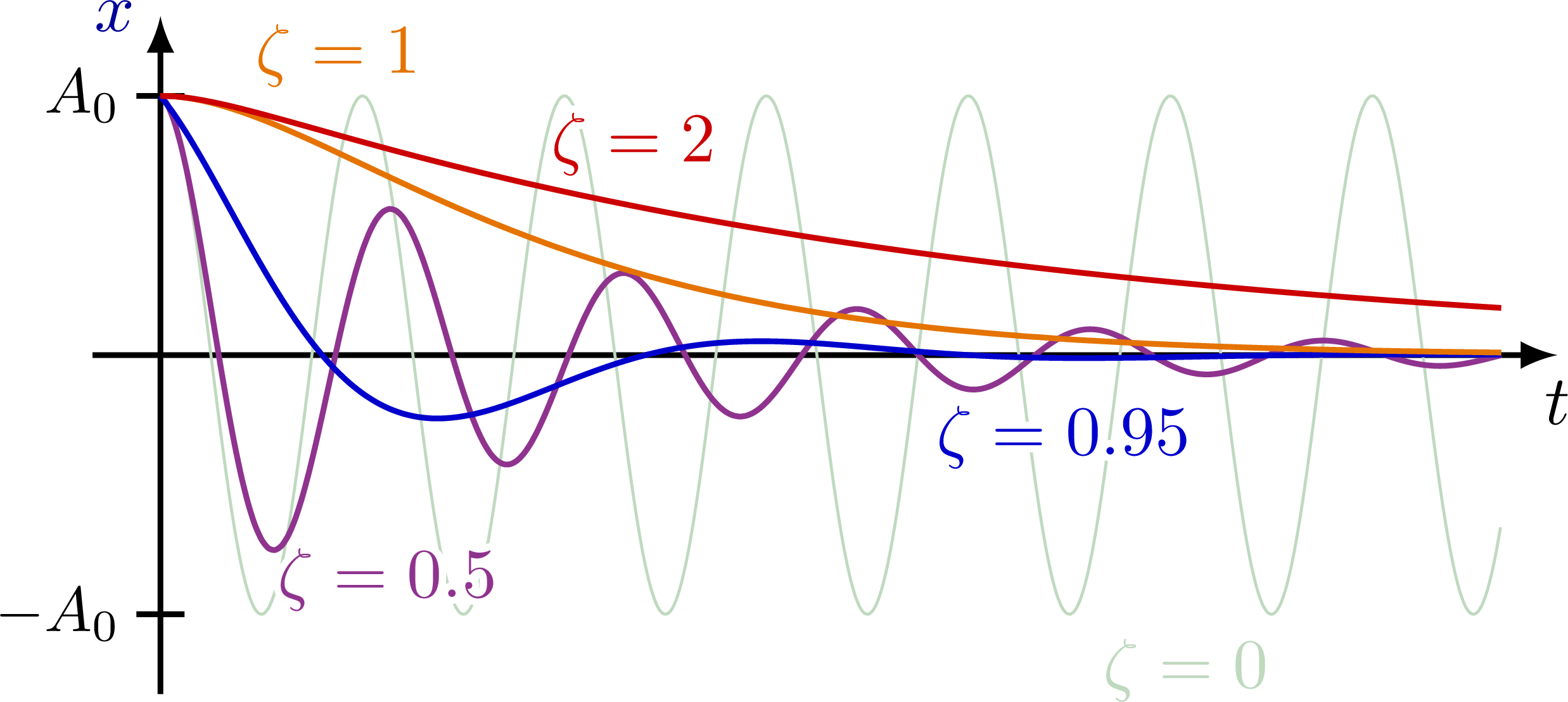
Different regimes of damped oscillators given by the damping ratio ζ: overdamped (red, ζ=2), critically damped (orange, ζ=1), underdamped (purple, ζ=0.5) and undamped (green, ζ=0).
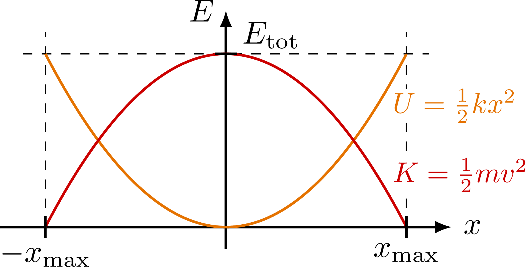
The kinetic (red), potential (orange), and total (dashed) energy of a simple harmonic oscillator as a function of displacement x are parabola:
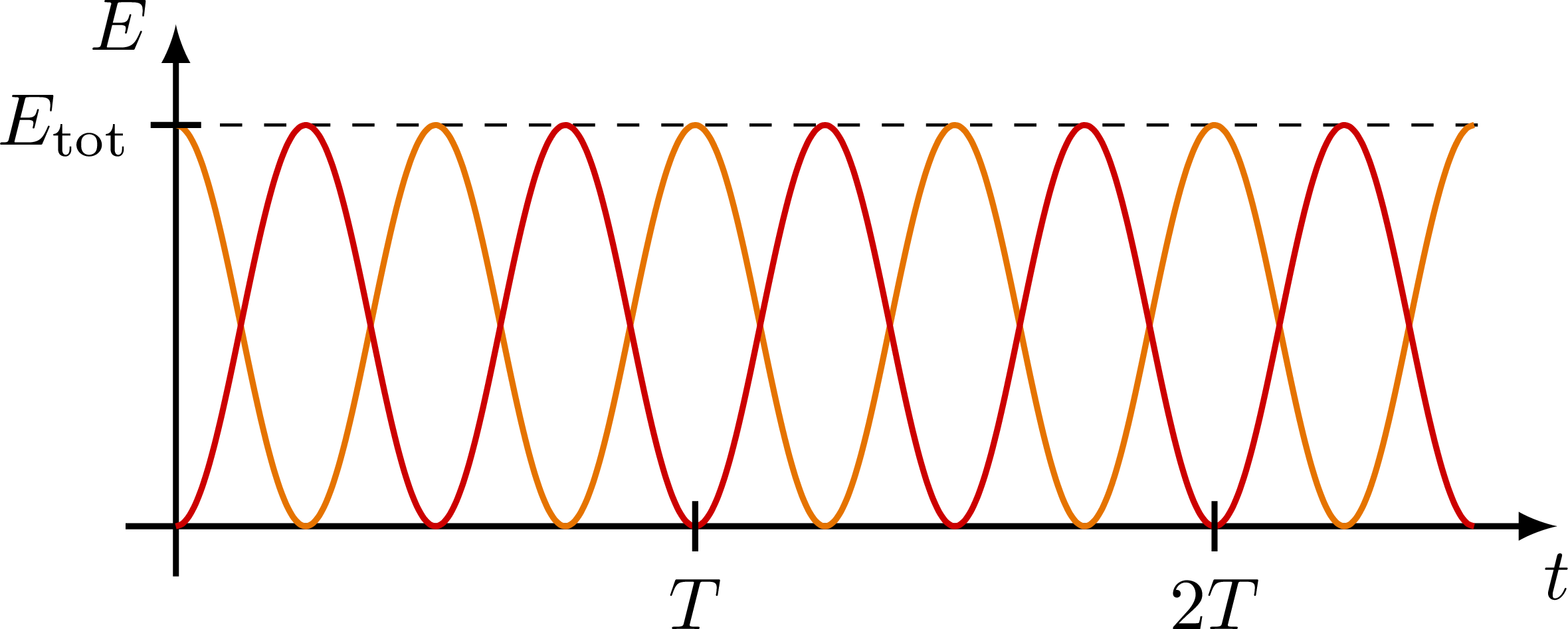
The kinetic (red), potential (orange), and total (dashed) energy of a simple harmonic oscillator as a function of time t are sine waves 90° out of phase.
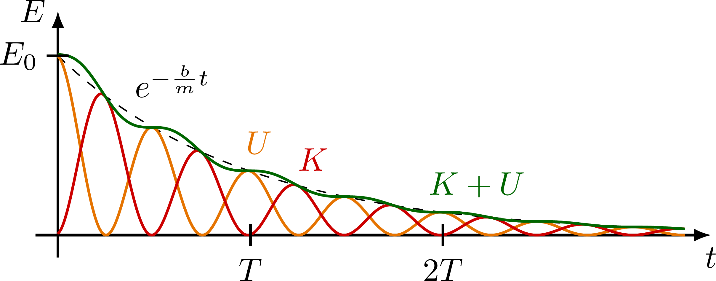
Kinetic (red), potential (orange), and total (green) energy of a damped harmonic oscillator as a function of time t. Note the averaged total energy (dashed) damps exponentially, and the actual total energy oscillates around it because energy is lost through motion.
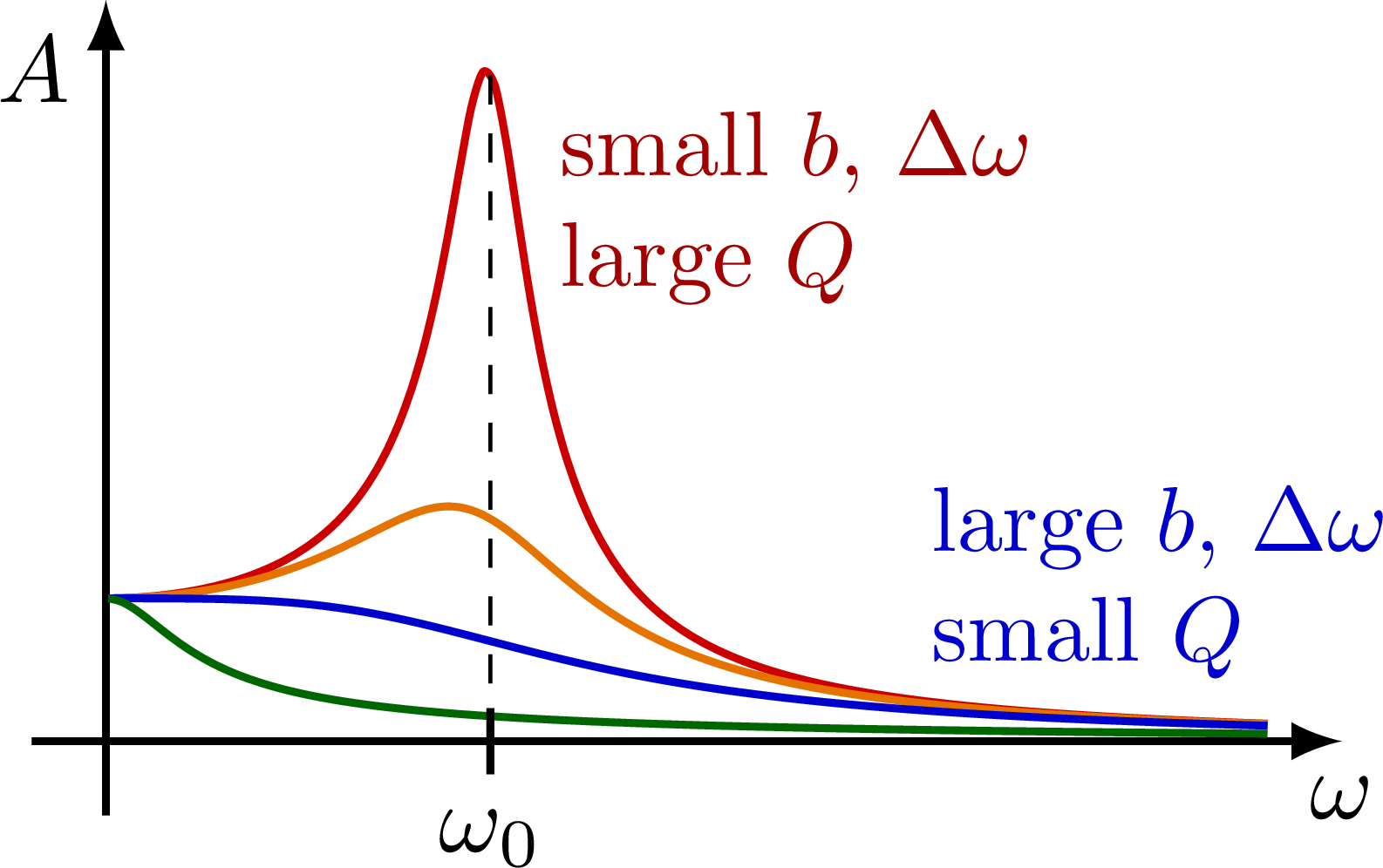
Amplitude of a driven harmonic oscillator to illustrate resonance with a natural frequency ω.
Edit and compile if you like:
% Author: Izaak Neutelings (October 2020)
% https://mathworld.wolfram.com/PhasePortrait.html
\documentclass[border=3pt,tikz]{standalone}
\usepackage{amsmath} % for \dfrac
\usepackage{physics,siunitx}
\usepackage{tikz,pgfplots}
\usepackage[outline]{contour} % glow around text
\contourlength{1.0pt}
\usetikzlibrary{angles,quotes} % for pic (angle labels)
\usetikzlibrary{arrows.meta}
\usetikzlibrary{decorations.markings}
%\usetikzlibrary{bending} % for arrow head angle
\tikzset{>=latex} % for LaTeX arrow head
\usepackage{xcolor}

\colorlet{xcol}{blue!60!black}
\colorlet{myred}{red!80!black}
\colorlet{myblue}{blue!80!black}
\colorlet{mygreen}{green!40!black}
\colorlet{myorange}{orange!90!black}
\colorlet{mypurple}{red!50!blue!90!black!80}
\colorlet{mydarkred}{myred!80!black}
\colorlet{mydarkblue}{myblue!80!black}
\tikzstyle{xline}=[xcol,thick]
\tikzstyle{width}=[{Latex[length=5,width=3]}-{Latex[length=5,width=3]},thick]
\tikzset{
  traj/.style 2 args={xline,postaction={decorate},decoration={markings,
    mark=at position #1 with {\arrow{<}},
    mark=at position #2 with {\arrow{<}}}
  }
}
\def\tick#1#2{\draw[thick] (#1)++(#2:0.12) --++ (#2-180:0.24)}
\def\N{100} % number of samples


\begin{document}


% CIRCLE on axis
\begin{tikzpicture}
  \def\A{1.4}
  \def\ang{40}
  \coordinate (O) at (0,0);
  \coordinate (X) at (\A,0);
  \coordinate (R) at (\ang:\A);
  \draw[->,thick] (-1.2*\A,0) -- (1.3*\A,0) node[below] {$x$};
  \draw[->,thick] (0,-1.2*\A) -- (0,1.3*\A) node[left] {$y$};
  \node[inner sep=2] (R') at (R) {};
  \draw[xcol] (0:\A) arc(0:90:\A);
  \draw[xcol] (110:\A) arc(110:340:\A);
  \draw[xcol,thick,line cap=round] (O) -- (R) node[midway,above=3] {$A$};
  \tick{0,-\A-0.008}{0}; %node[left=-1,scale=1] {$A$};
  \tick{0, \A+0.008}{0} node[left=-2,scale=1] {$A$};
  \tick{-\A-0.008,0}{90}; %node[below=-1,scale=1] {$A$};
  \tick{ \A+0.008,0}{90} node[left=0.5,below=-2,scale=1] {$A$};
  \draw pic[->,"$\omega t$",xcol,draw=xcol,angle radius=19,angle eccentricity=1.4] {angle=X--O--R};
  \fill[myred!50!black] (R) circle (0.07);
  \draw[->,mygreen!80!black] (\ang+5:1.2*\A) arc(\ang+5:\ang+35:0.9*\A) node[midway,above right=-1] {$\omega$};
\end{tikzpicture}


% CIRCLE on axis + phase
\begin{tikzpicture}
  \def\A{1.4}
  \def\ang{30}
  \def\phase{19}
  \coordinate (O) at (0,0);
  \coordinate (X) at (\A,0);
  \coordinate (R0) at (\phase:\A);
  \coordinate (R) at (\ang+\phase:\A);
  \draw[->,thick] (-1.2*\A,0) -- (1.3*\A,0) node[below] {$x$};
  \draw[->,thick] (0,-1.2*\A) -- (0,1.3*\A) node[left] {$y$};
  \node[inner sep=2] (R') at (R) {};
  \draw[xcol] (0:\A) arc(0:90:\A);
  \draw[xcol] (110:\A) arc(110:340:\A);
  \draw[xcol,thick,line cap=round] (O) -- (R) node[midway,above=3] {$A$};
  \draw[xcol,thin] (O) -- (R0);
  \tick{0,-\A}{0}; %node[left=-1,scale=1] {$A$};
  \tick{0, \A}{0} node[left=-2,scale=1] {$A$};
  \tick{-\A,0}{90}; %node[below=-1,scale=1] {$A$};
  \tick{ \A,0}{90} node[left=0.5,below=-2,scale=1] {$A$};
  \draw pic[->,"$\phi$",xcol,draw=xcol,angle radius=27,angle eccentricity=1.23] {angle=X--O--R0};
  \draw pic[->,"$\omega t$",xcol,draw=xcol,angle radius=21,angle eccentricity=1.45] {angle=R0--O--R};
  \fill[myred!50!black] (R) circle (0.07);
  \draw[->,mygreen!80!black] (\ang+\phase+5:1.2*\A) arc(\ang+\phase+5:\ang+\phase+35:0.9*\A) node[midway,above right=-1] {$\omega$};
\end{tikzpicture}


% COS
\def\xmax{6.6} % max x axis
\def\ymax{1.2} % max y axis
\def\A{0.8}    % amplitude
\def\om{(2.55*360/(0.94*\xmax))} % angular frequency in degrees
\begin{tikzpicture}

  % AXIS
  \draw[->,thick] (0,-\ymax) -- (0,\ymax) node[left,xcol] {$x$};
  \draw[->,thick] (-0.2*\ymax,0) -- (\xmax,0) node[below] {$t$};
  \draw[dashed] ({360/\om},1.2*\A) --++ (0,-2.7*\A);
  \tick{0,\A}{0} node[left=-1,scale=0.9] {$A$};
  \tick{{360/\om},0}{90} node[below,scale=0.9] {\contour{white}{$T$}};
  \tick{{720/\om},0}{90} node[below,scale=0.9] {$2T$};
  \draw[<->]
    (0,-1.35*\A) --++ ({360/\om},0)
    node[midway,fill=white,inner sep=1,scale=0.9] {$T = 2\pi/\omega$};

  % PLOT
  \draw[xline,samples=\N,smooth,variable=\x,domain=0:0.94*\xmax]
    plot(\x,{\A*cos(\om*\x)});
  %\node[xcol,above=2,right=4] at ({720/\om},\A) {$x(t)=A\cos(\omega t)$};

\end{tikzpicture}


% COS - phase
\begin{tikzpicture}
  \def\phase{60}

  % AXIS
  \draw[->,thick] (0,-\ymax) -- (0,\ymax) node[left,xcol] {$x$};
  \draw[->,thick] (-0.2*\ymax,0) -- (\xmax,0) node[below] {$t$};
  \tick{0,\A}{0} node[left=-1,scale=0.9] {$A$};
  \tick{{\phase/\om},0}{90} node[below,scale=0.9] {$t_0$};
  \draw[dashed] ({\phase/\om},0) --++ (0,1.2*\A);
  \draw[dashed] ({180/\om},-1.3*\A) --++ (0,1.5*\A);
  \draw[dashed] ({(180+\phase)/\om},-1.3*\A) --++ (0,1.5*\A);
  \draw[->]
    ({180/\om},-1.25*\A) --++ ({\phase/\om},0)
    node[midway,below,scale=0.9] {$t_0 = \phi/\omega$};

  % PLOT
  \draw[xcol!30,thin,dashed,samples=\N,smooth,variable=\x,domain=0:0.94*\xmax]
    plot(\x,{\A*cos(\om*\x)});
  \draw[xline,samples=\N,smooth,variable=\x,domain=0:0.94*\xmax]
    plot(\x,{\A*cos(\om*\x-\phase)});
  \tick{{(360+\phase)/\om},0}{90} node[below,scale=0.9] {\contour{white}{$t_0+T$}};
  \tick{{(720+\phase)/\om},0}{90} node[below,scale=0.9] {\contour{white}{$t_0+2T$}};

\end{tikzpicture}


% COS - phase - vertical shift
\begin{tikzpicture}
  \def\phase{60}
  \def\C{0.5*\A}

  % AXIS
  \draw[->,thick] (0,\C-\ymax) -- (0,\C+1.05*\ymax) node[left,xcol] {$y$};
  \draw[->,thick] (-0.2*\ymax,0) -- (\xmax,0) node[below] {$t$};
  \tick{0,\C+\A}{0} node[left=-1,scale=0.9] {$A+y_0$};
  \tick{0,\C-\A}{0} node[left=-1,scale=0.9] {$-A+y_0$};
  \tick{0,\C}{0} node[left=-1,scale=0.9] {$y_0$};

  % PLOT
  \draw[dashed] (0,\C) --++ (0.95*\xmax,0);
  \draw[xline,samples=\N,smooth,variable=\x,domain=0:0.94*\xmax]
    plot(\x,{\C+\A*cos(\om*\x-\phase)});
  %\tick{{(360+\phase)/\om},0}{90} node[below,scale=0.9] {\contour{white}{$t_0+T$}};
  %\tick{{(720+\phase)/\om},0}{90} node[below,scale=0.9] {\contour{white}{$t_0+2T$}};

\end{tikzpicture}


% COS - damped
\begin{tikzpicture}
  \def\xmax{7.0} % max x axis
  \def\ymax{1.7}
  \def\A{1.3}
  \def\om{(5.3*360/(0.94*\xmax))}
  \def\t{1800/(0.94*\xmax)}
  \def\T{2.5}

  % AXIS
  \draw[->,thick] (0,-\ymax) -- (0,\ymax) node[left,xcol] {$x$};
  \draw[->,thick] (-0.2*\ymax,0) -- (\xmax,0) node[below] {$t$};
  \tick{0,\A}{0} node[left=-1,scale=0.9] {$A_0$};
  \tick{0,-\A}{0} node[left=-1,scale=0.9] {$-A_0$};

  % PLOT
  \draw[dashed,samples=\N,smooth,variable=\t,domain=0:0.96*\xmax]
    plot(\t,{\A*exp(-\t/\T)}) plot(\t,{-\A*exp(-\t/\T)});
  \draw[xline,samples=100+\N,smooth,variable=\t,domain=0:0.96*\xmax]
    plot(\t,{\A*exp(-\t/\T)*cos(\om*\t)});
  \node[above=4] at (0.18*\xmax,{\A*exp(-0.18*\xmax/\T)}) {$e^{-\frac{b}{2m}t}$};

\end{tikzpicture}


% COS - overdamped
% https://en.wikipedia.org/wiki/Harmonic_oscillator#Universal_oscillator_equation
% https://brilliant.org/wiki/damped-harmonic-oscillators/
% https://beltoforion.de/en/harmonic_oscillator/
% http://hyperphysics.phy-astr.gsu.edu/hbase/oscda.html#c1
% http://hyperphysics.phy-astr.gsu.edu/hbase/oscda2.html#c1
% https://ocw.mit.edu/courses/mathematics/18-03sc-differential-equations-fall-2011/unit-ii-second-order-constant-coefficient-linear-equations/damped-harmonic-oscillators/MIT18_03SCF11_s13_2text.pdf
\begin{tikzpicture}
  \def\xmax{7.0} % max x axis
  \def\ymax{1.7} % max y axis
  \def\A{1.3}
  \def\om{(6.5/(0.94*\xmax))} % natural omega_0
  \def\Za{0.50} % zeta underdamped 1
  \def\Zb{0.95} % zeta underdamped 2
  \def\Zc{1.00} % zeta critically damped
  \def\Zd{2.00} % zeta overdamped
  \def\Ga{(\Za*\om)} % gamma underdamped 1
  \def\Gb{(\Zb*\om)} % gamma underdamped 2
  \def\Gc{\om}       % gamma critically damped
  \def\Gd{(\Zd*\om)} % gamma overdamped
  \def\Wa{(\om*sqrt(1-\Za*\Za)}  % omega underdamped 1
  \def\Wb{(\om*sqrt(1-\Zb*\Zb)}  % omega underdamped 2
  \def\Wd{(\om*sqrt(\Zd*\Zd-1))} % omega overdamped

  % AXIS
  \draw[->,thick] (0,-\ymax) -- (0,\ymax) node[left,xcol] {$x$};
  \draw[->,thick] (-0.2*\ymax,0) -- (\xmax,0) node[below] {$t$};
  \tick{0,\A}{0} node[left=-1,scale=0.9] {$A_0$};
  \tick{0,-\A}{0} node[left=-1,scale=0.9] {$-A_0$};

  % PLOT
  \draw[xline,mygreen!25,thin,samples=200+\N,smooth,variable=\t,domain=0:0.96*\xmax]
    plot(\t,{\A*cos(360*\om*\t)});
  \draw[xline,mypurple,samples=100+\N,smooth,variable=\t,domain=0:0.96*\xmax]
    plot(\t,{\A*exp(-\Ga*\t)*cos(360*\Wa*\t)});
  \draw[xline,myblue,samples=\N,smooth,variable=\t,domain=0:0.96*\xmax]
    plot(\t,{\A*exp(-\Gb*\t)*cos(360*\Wb*\t)});
  \draw[xline,myorange,samples=\N,smooth,variable=\t,domain=0:0.96*\xmax]
    plot(\t,{\A*(1+\Gc*\t)*exp(-\Gc*\t)});
  \draw[xline,myred,samples=\N,smooth,variable=\t,domain=0:0.96*\xmax]
    plot(\t,{\A/2*( (1+\Gd/\Wd)*exp((\Wd-\Gd)*\t) + (1-\Gd/\Wd)*exp(-(\Wd+\Gd)*\t))});
  %\node[above=4] at (0.15*\xmax,{\A*exp(-0.15*\xmax/\T)}) {$e^{-\frac{b}{2m}t}$};

  % NODES
  \node[below,mygreen!25] at ({5.20*\om},-1.00*\A) {$\zeta=0$};
  \node[below,mypurple]   at ({1.15*\om},-0.65*\A) {\contour{white}{$\zeta=0.5$}};
  \node[below,myblue]     at ({4.58*\om},-0.10*\A) {\contour{white}{$\zeta=0.95$}};
  \node[above,myorange]   at ({0.90*\om}, 0.94*\A) {$\zeta=1$};
  \node[above,myred]      at ({2.40*\om}, 0.60*\A) {\contour{white}{$\zeta=2$}};

\end{tikzpicture}


% ENERGY vs. x
\begin{tikzpicture}
  \def\xmax{2.5}    % max x axis
  \def\ymax{2.4}    % max y axis
  \def\A{0.8*\xmax} % maximum extension
  \def\E{0.8*\ymax} % maximum total energy

  % AXIS
  \draw[->,thick] (0,-0.1*\ymax) -- (0,\ymax) node[left] {$E$};
  \draw[->,thick] (-\xmax,0) -- (\xmax,0) node[right] {$x$};
  \draw[dashed] (-\A,0) --++ (0,0.9*\ymax);
  \draw[dashed] ( \A,0) --++ (0,0.9*\ymax);
  \draw[dashed] (-0.9*\xmax,\E) -- (0.9*\xmax,\E);

  % PLOT
  \draw[xline,myorange,samples=\N,smooth,variable=\x,domain=-\A:\A]
    plot(\x,{\E/(\A*\A)*\x*\x)});
  \draw[xline,myred,samples=\N,smooth,variable=\x,domain=-\A:\A]
    plot(\x,{\E-\E/(\A*\A)*\x*\x)});
  \tick{0,\E}{180} node[above right=-2,scale=1] {$E_\text{tot}$};
  \tick{-\A,0}{90} node[below=-2,scale=1] {$-x_\text{max}$};
  \tick{\A,0}{90} node[below=-2,scale=1] {$x_\text{max}$};
  \node[myorange,right,fill=white,inner sep=0,scale=0.9] at (0.92*\A,0.7*\E) {$U = \frac{1}{2}kx^2$};
  \node[myred,right,fill=white,inner sep=0,scale=0.9] at (0.92*\A,0.3*\E) {$K = \frac{1}{2}mv^2$};

\end{tikzpicture}


% ENERGY vs. t
\begin{tikzpicture}
  \def\ymax{2.4} % max y axis
  \def\A{0.8*\ymax} % maximum extension
  \def\om{(2.5*360/(0.94*\xmax))} % angular frequency in degrees

  % AXIS
  \draw[->,thick] (0,-0.1*\ymax) -- (0,\ymax) node[left] {$E$};
  \draw[->,thick] (-0.1*\ymax,0) -- (\xmax,0) node[below] {$t$};
  \draw[dashed] (0,\A) -- (0.95*\xmax,\A);

  % PLOT
  \draw[xline,myorange,samples=100+\N,smooth,variable=\x,domain=0:0.94*\xmax]
    plot(\x,{\A*cos(\om*\x)^2});
  \draw[xline,myred,samples=100+\N,smooth,variable=\x,domain=0:0.94*\xmax]
    plot(\x,{\A*sin(\om*\x)^2});
  \tick{0,\A}{0} node[left=-1,scale=1] {$E_\text{tot}$};
  \tick{{360/\om},0}{90} node[below,scale=1] {$T$};
  \tick{{720/\om},0}{90} node[below,scale=1] {$2T$};

\end{tikzpicture}


% ENERGY vs. t - damped
\begin{tikzpicture}
  \def\xmax{7.0} % max x axis
  \def\ymax{2.4} % max y axis
  \def\A{0.8*\ymax} % maximum extension
  \def\T{4.0}    % decay constant tau
  %\def\om{(2.5*360/(0.94*\xmax))} % angular frequency in degrees
  \def\om{(3.2*2*pi/(0.94*\xmax))} % angular frequency in radians
  \def\W{(sqrt((\om)^2-1/\T/\T))} % omega underdamped

  % AXIS
  \draw[->,thick] (0,-0.1*\ymax) -- (0,\ymax) node[left] {$E$};
  \draw[->,thick] (-0.1*\ymax,0) -- (\xmax,0) node[below] {$t$};

  % PLOT
  \draw[dashed,samples=\N,smooth,variable=\x,domain=0:0.96*\xmax]
    plot(\x,{\A*exp(-2*\x/\T)});
  \draw[xline,myorange,samples=100+\N,smooth,variable=\x,domain=0:0.96*\xmax]
    plot(\x,{\A*exp(-2*\x/\T)*cos(180/pi*\W*\x)^2});
  \draw[xline,myred,samples=100+\N,smooth,variable=\x,domain=0:0.96*\xmax]
    %plot(\x,{\A*exp(-\x/\T)*sin(180/pi*\W*\x)^2});
    plot(\x,{\A*exp(-2*\x/\T)*( 1/\T/\om*cos(180/pi*\W*\x) + \W/\om*sin(180/pi*\W*\x) )^2});
  \draw[xline,mygreen,samples=100+\N,smooth,variable=\x,domain=0:0.96*\xmax]
    plot(\x,{\A*exp(-2*\x/\T)*(cos(180/pi*\W*\x)^2 + ( 1/\T/\om*cos(180/pi*\W*\x) + \W/\om*sin(180/pi*\W*\x) )^2 )});
  \node[above right=0] at (0.1*\xmax,{\A*exp(-2*0.1*\xmax/\T)}) {$e^{-\frac{b}{m}t}$};
  \node[above right=0,myorange] at (0.27*\xmax,{\A*exp(-2*0.27*\xmax/\T)}) {$U$};
  \node[above right=0,myred] at (0.35*\xmax,{\A*exp(-2*0.35*\xmax/\T)}) {$K$};
  \node[above right=0,mygreen] at (0.55*\xmax,{\A*exp(-2*0.55*\xmax/\T)}) {$K+U$};
  \tick{0,\A}{0} node[left=-1,scale=1] {$E_0$};
  \tick{{2*pi/\W},0}{90} node[below,scale=1] {$T$};
  \tick{{4*pi/\W},0}{90} node[below,scale=1] {$2T$};

\end{tikzpicture}


% RESONANCE
\begin{tikzpicture}
  \def\xmax{4.5}
  \def\ymax{2.7}
  \def\c{1.4}        % natural frequency
  \def\A{0.90*\ymax} % amplitude
  \def\ba{0.3}       % drag coefficient 1
  \def\bb{0.9}       % drag coefficient 2
  \def\bc{2.0}       % drag coefficient 3
  \def\bd{8.0}       % drag coefficient 4
  \coordinate (O) at (0,0);
  \coordinate (X) at (\xmax,0);
  \coordinate (Y) at (0,\ymax);
  \coordinate (C) at (\c,0);

  % AXIS
  \draw[->,thick]
    (-0.1*\ymax,0) -- (\xmax,0) node[below] {$\omega$};
  \draw[->,thick]
    (0,-0.1*\ymax) -- (0,\ymax) node[below left] {$A$}; %\langle{P}\rangle

  % PLOT
  \draw[xline,myred,samples=\N,smooth,variable=\x,domain=0.01:0.94*\xmax]
    plot(\x,{\A*\ba*\c/sqrt((\c*\c-\x*\x)^2 + (\ba*\x)^2 )});
  \draw[xline,myorange,samples=\N,smooth,variable=\x,domain=0.01:0.94*\xmax]
    plot(\x,{\A*\ba*\c/sqrt((\c*\c-\x*\x)^2 + (\bb*\x)^2 )});
  \draw[xline,myblue,samples=\N,smooth,variable=\x,domain=0.01:0.94*\xmax]
    plot(\x,{\A*\ba*\c/sqrt((\c*\c-\x*\x)^2 + (\bc*\x)^2 )});
  \draw[xline,mygreen,samples=\N,smooth,variable=\x,domain=0.01:0.94*\xmax]
    plot(\x,{\A*\ba*\c/sqrt((\c*\c-\x*\x)^2 + (\bd*\x)^2 )});
  \node[mydarkred,align=left,right,scale=0.95] at ({0.26*(\c+\xmax)},0.8*\A) {small $b$, $\Delta\omega$\\large $Q$};
  \node[myblue,align=left,above,scale=0.95] at ({0.65*(\c+\xmax)},0.3*\A*\ba/\bc) {large $b$, $\Delta\omega$\\small $Q$};
  \draw[dashed,thin] (C) --++ (0,\A);
  \tick{C}{90} node[below] {$\omega_0$};

  % WIDTH
  %\draw[<->,thick] ({\c/(2*\Q)*(-1+sqrt(1+4*\Q^2))},\A/2) -- ({\c/(2*\Q)*(1+sqrt(1+4*\Q^2))},\A/2);
  %\draw[width,myblue!80!black]
  %  ({\c/(2*\q)*(-1+sqrt(1+4*\q^2))},\a/2) --++ (\c/\q,0) node[midway,above] {$\Delta \omega$};
  %\draw[width,mydarkred]
  %  ({\c/sqrt(2*\Q)*(-1+sqrt(1+4*\Q^2))},\A/2) --++ {(\c/sqrt(\Q)},0)
  %  node[midway,left=0.8,above,scale=0.9] {\contour{white}{$\Delta \omega$}};

\end{tikzpicture}


\end{document}
Click to download: dynamics_oscillator.tex • dynamics_oscillator.pdf
Open in Overleaf: dynamics_oscillator.tex


