")


Basic physics of a (physical) pendulum. The plots of the exact solution with an arbitrarily large amplitude is inspired by this article, and Wikipedia.
For more on the pendulums, please see the “pendulum” tag . For more on the small-angle approximation, please see the “Taylor expansion” tag.
These figures are used in Ben Kilminster’s lecture notes for PHY111.
Simple pendulum:
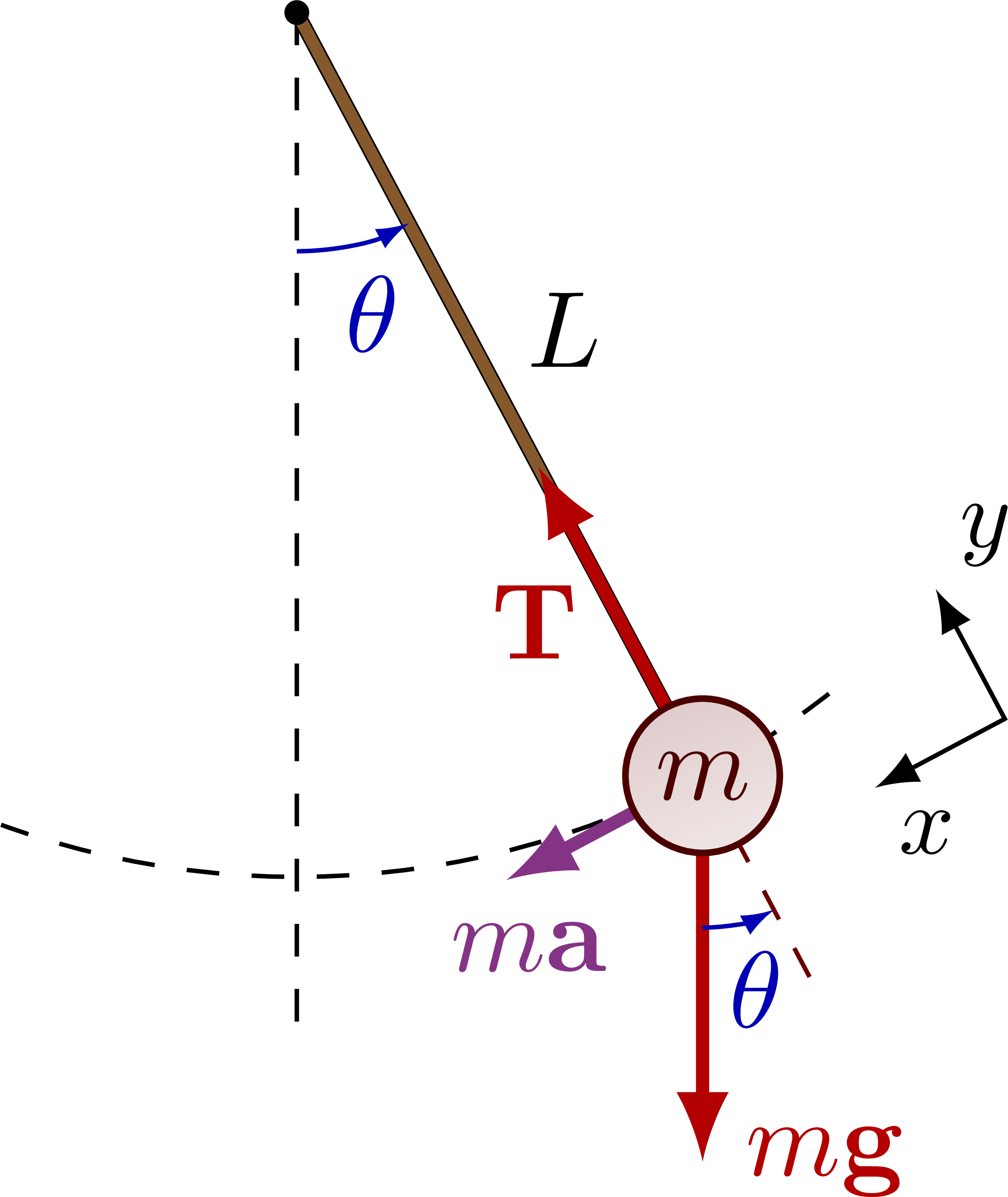
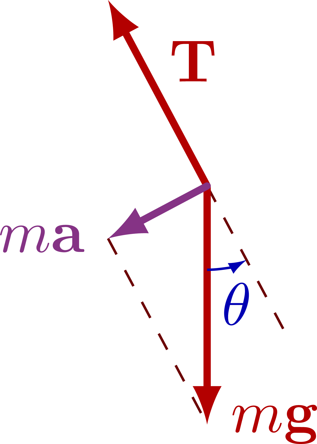
Force diagram of a pendulum to apply Newton’s second law:
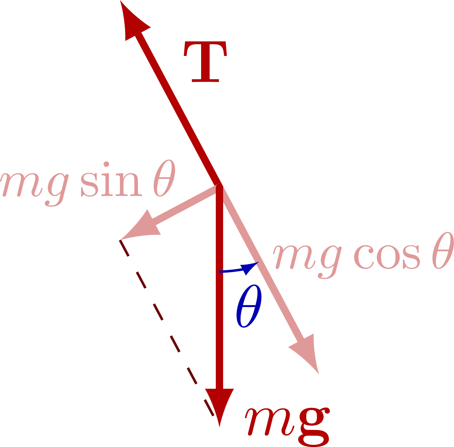
Force diagram of a pendulum, breaking down the force components:
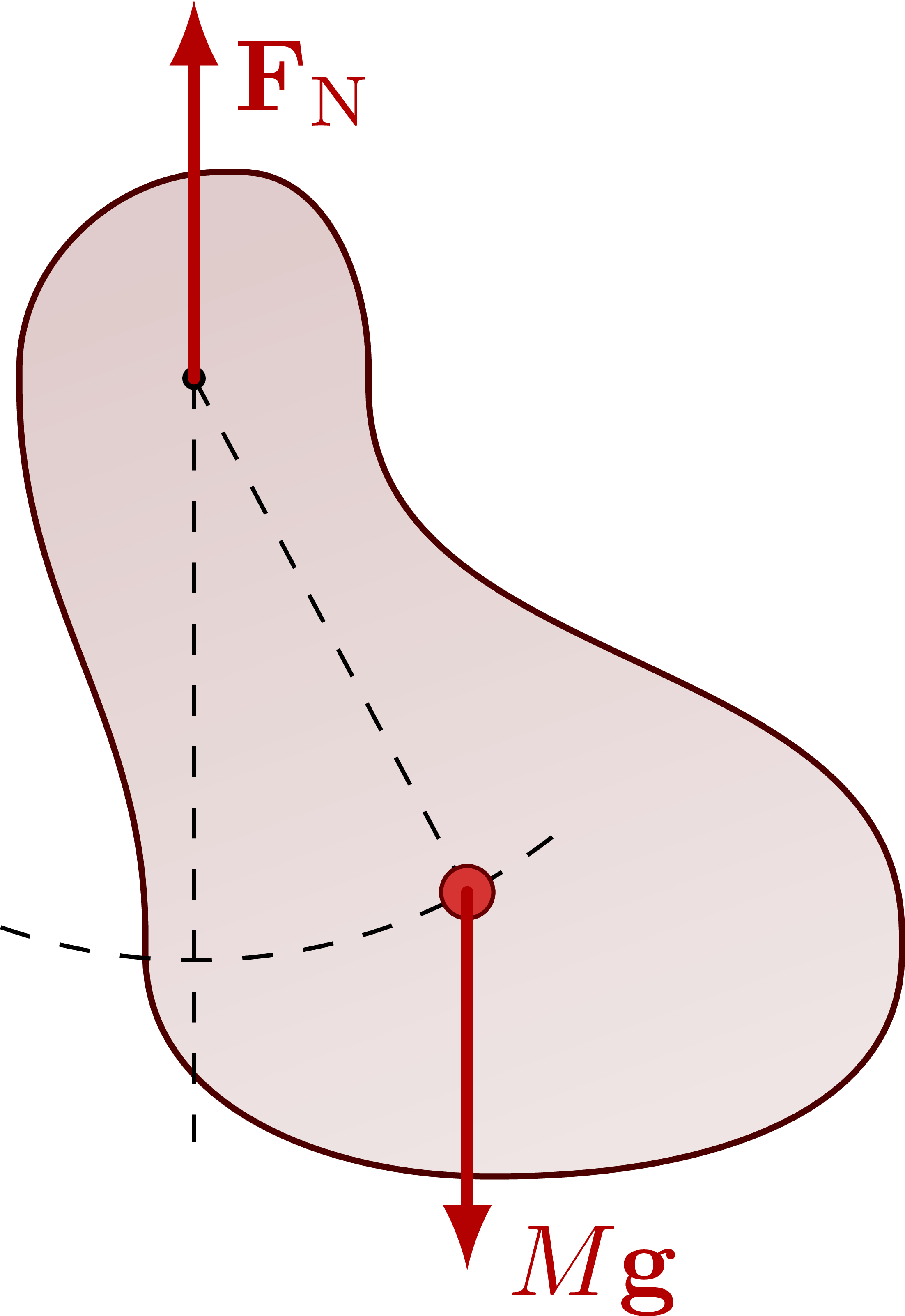
Physical pendulum:
Exact solution
The curves in the figures below are created using numerical data produced by these MATLAB scripts. The data needs to be loaded via these text files to compile this part of the code. A full working setup with input files is also available from this zip file.
Closed solutions (bounded)
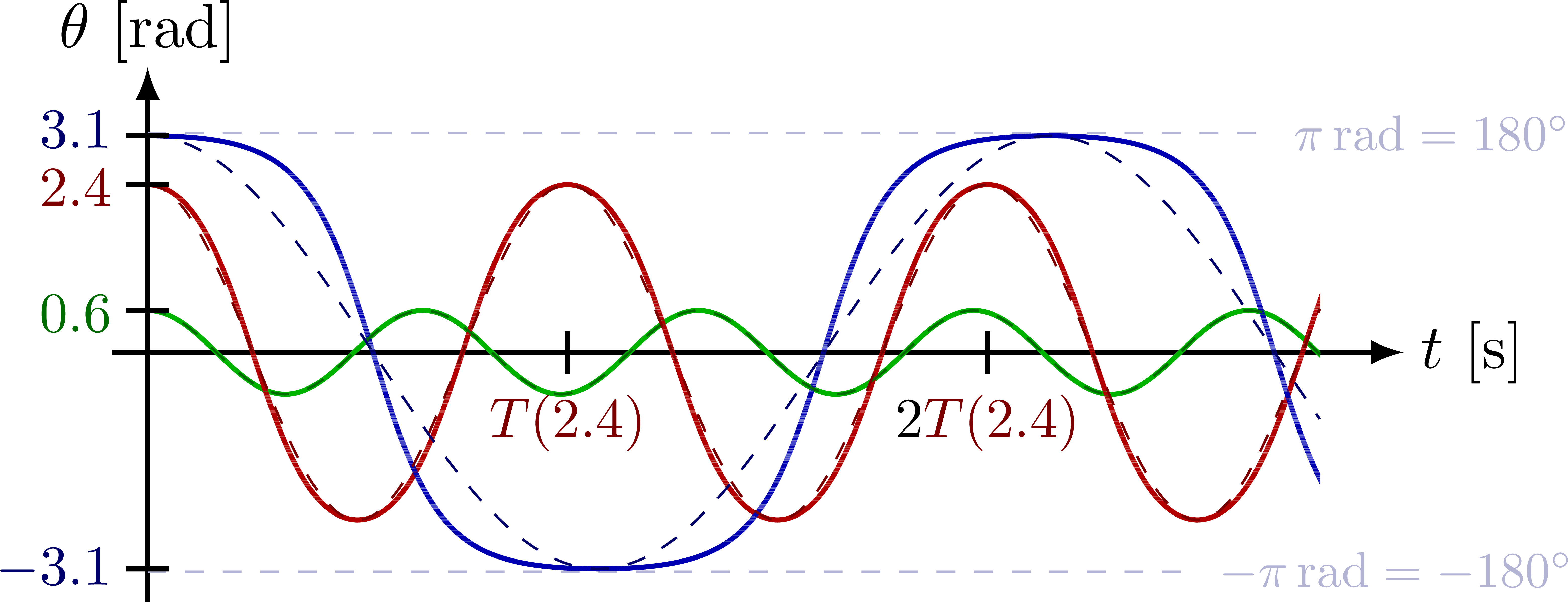
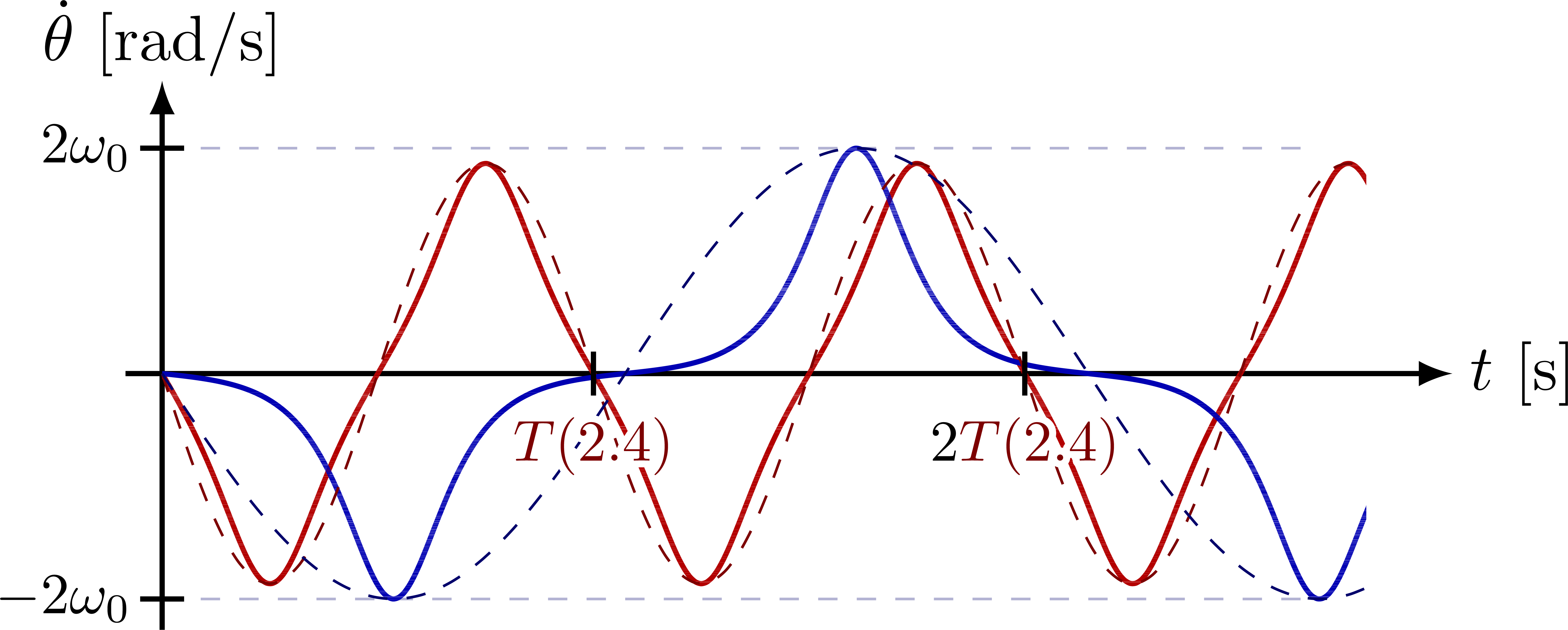
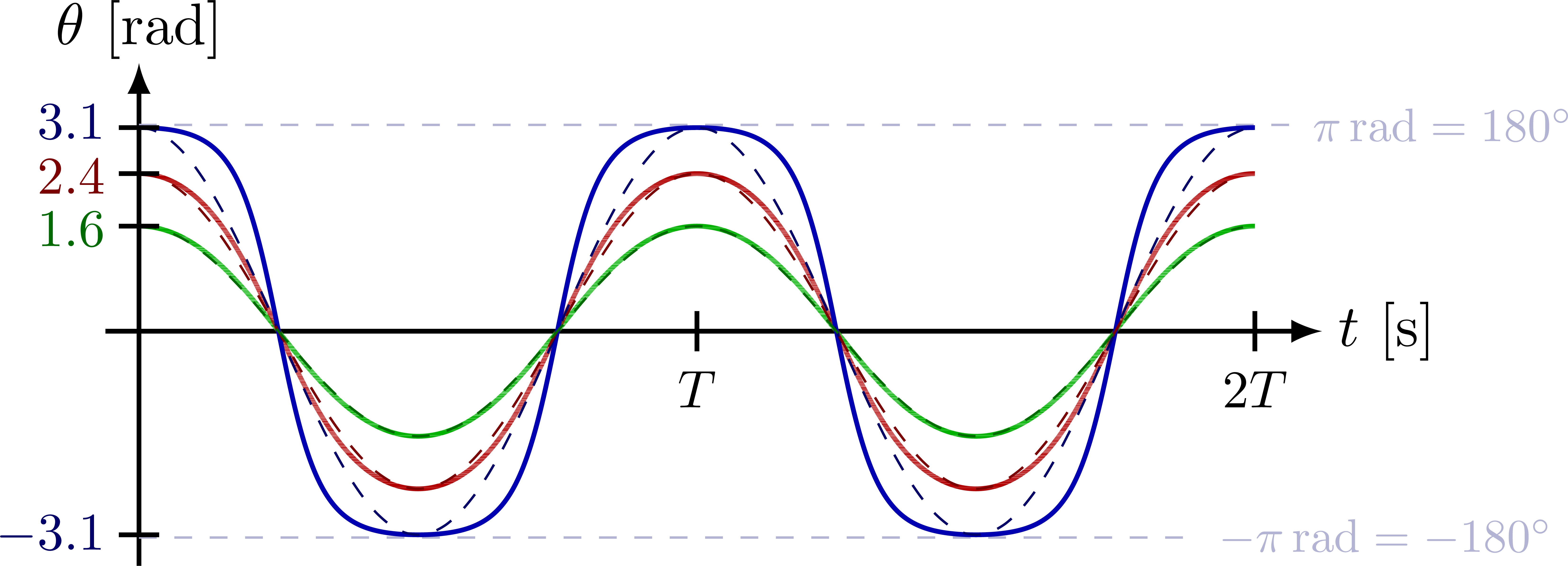
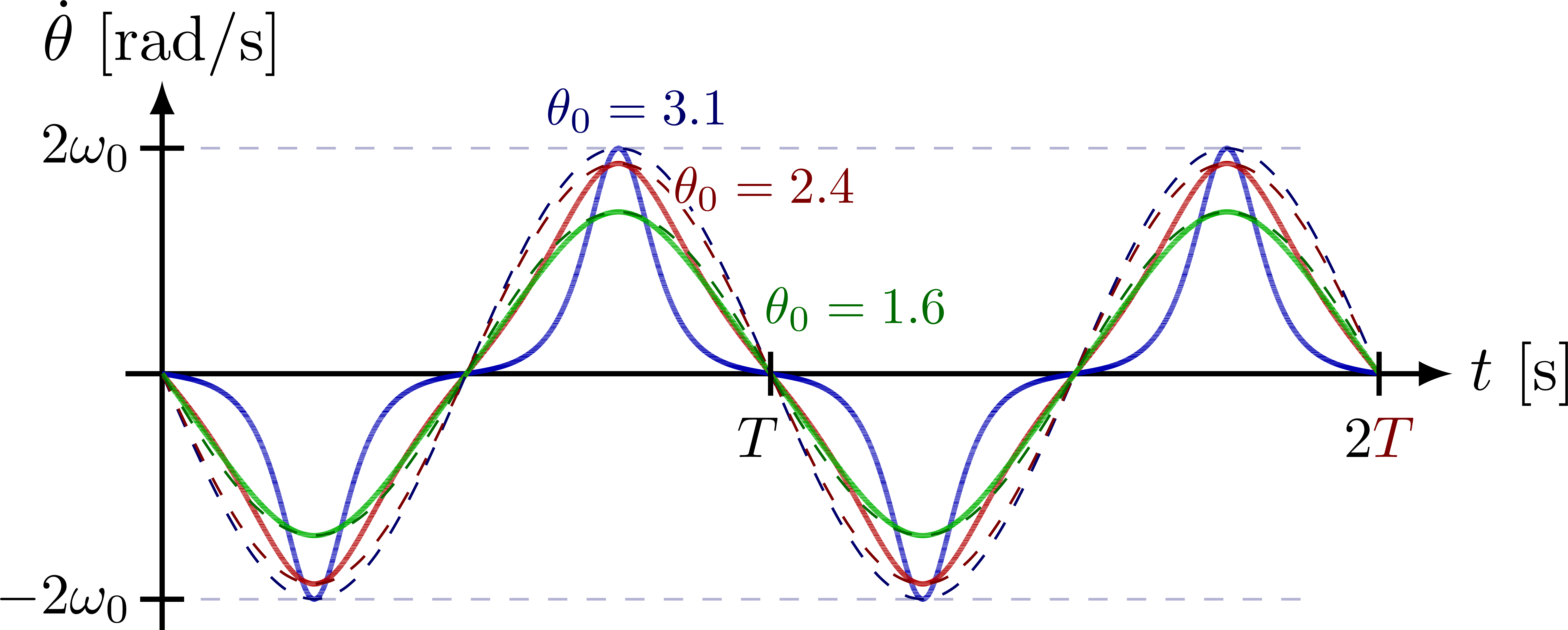
Comparison of exact solution of a pendulum to a sine with the same period.
Please note that the ideal solution from the small-angle approximation actually has a fixed period T_0. The dashed lines are rescales along the time axis to compare the shape of the exact solutions to cosines.
Angle θ of the pendulum versus time for several amplitudes:
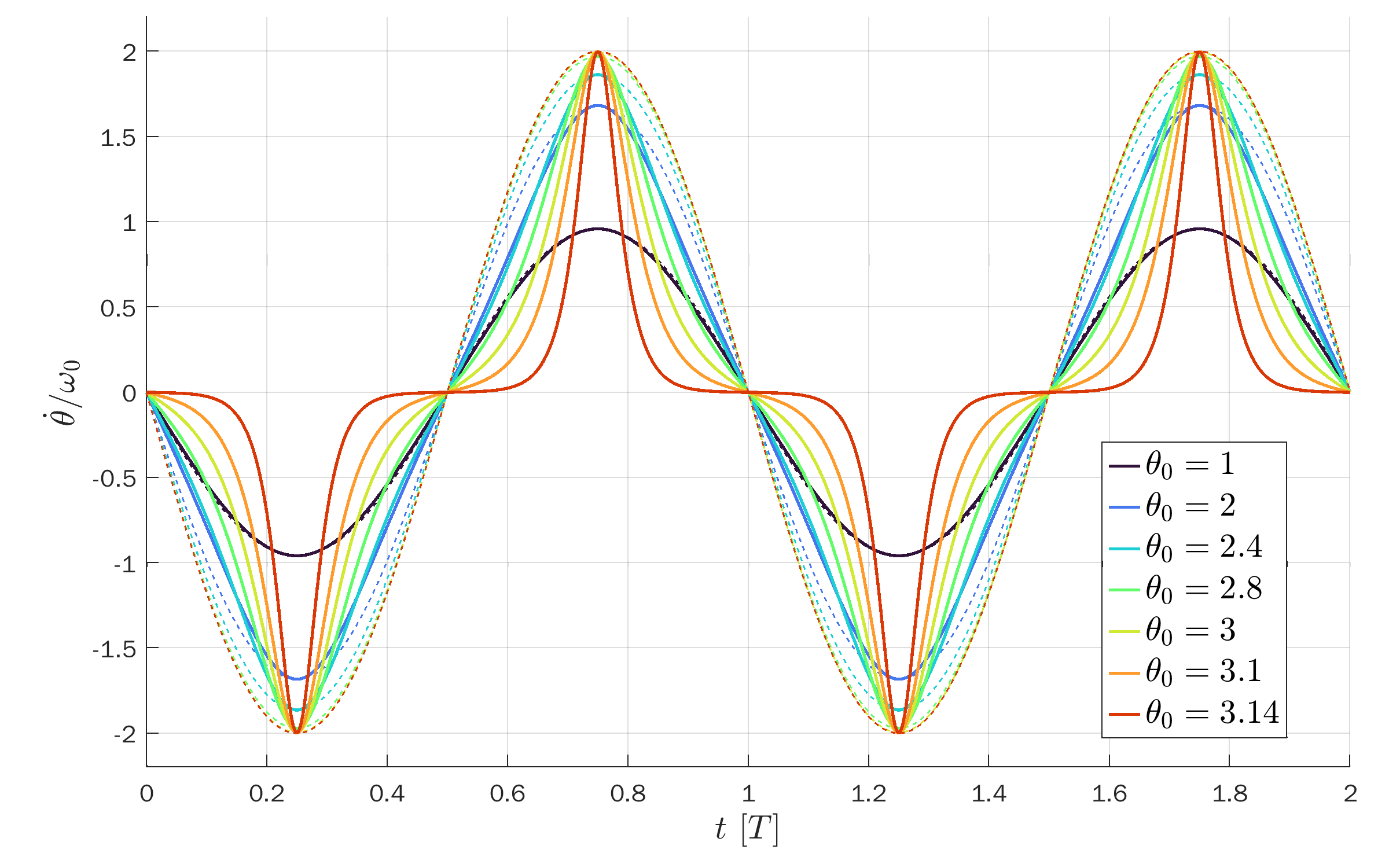
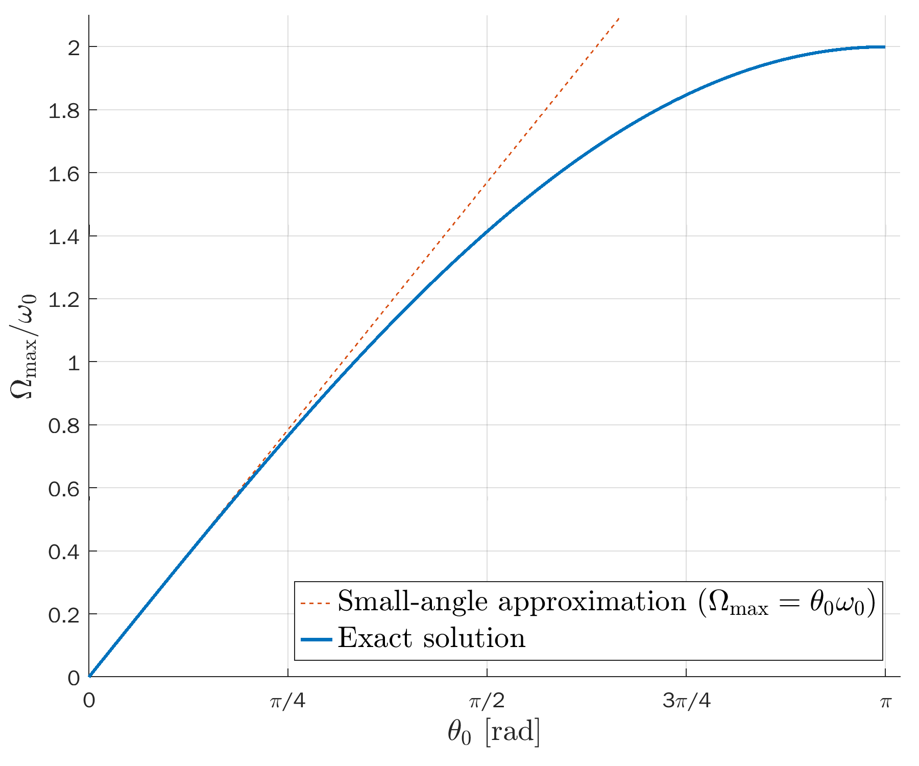
Angular velocity (first derivative of the pendulum’s angle):
All curves are plotted versus t/T so the peaks coincide:
Angular velocity versus t/T so the peaks coincide:
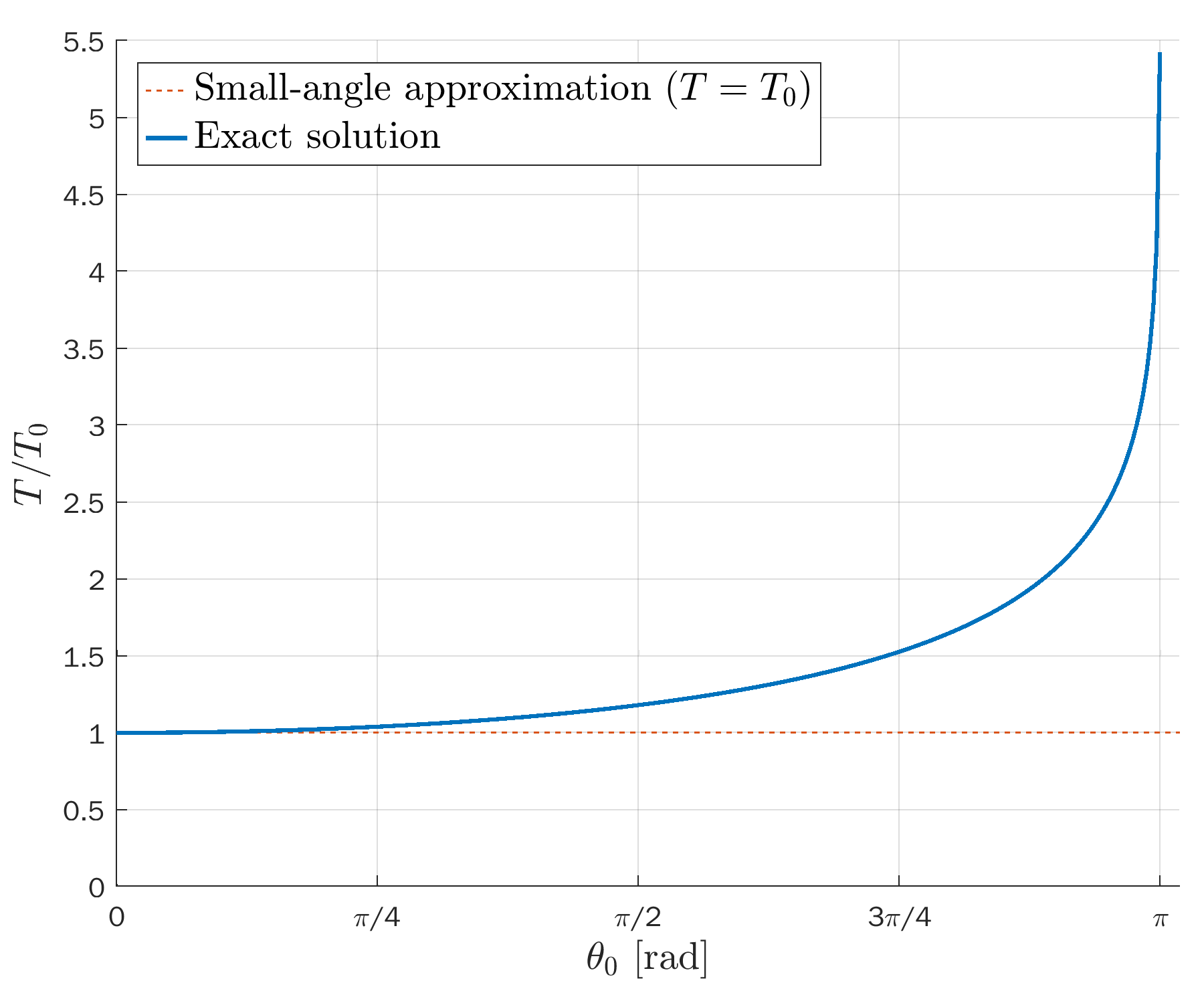
Ratio between real and ideal period of a pendulum, T/T_0, as a function of the angular amplitude (see this Wikipedia section).
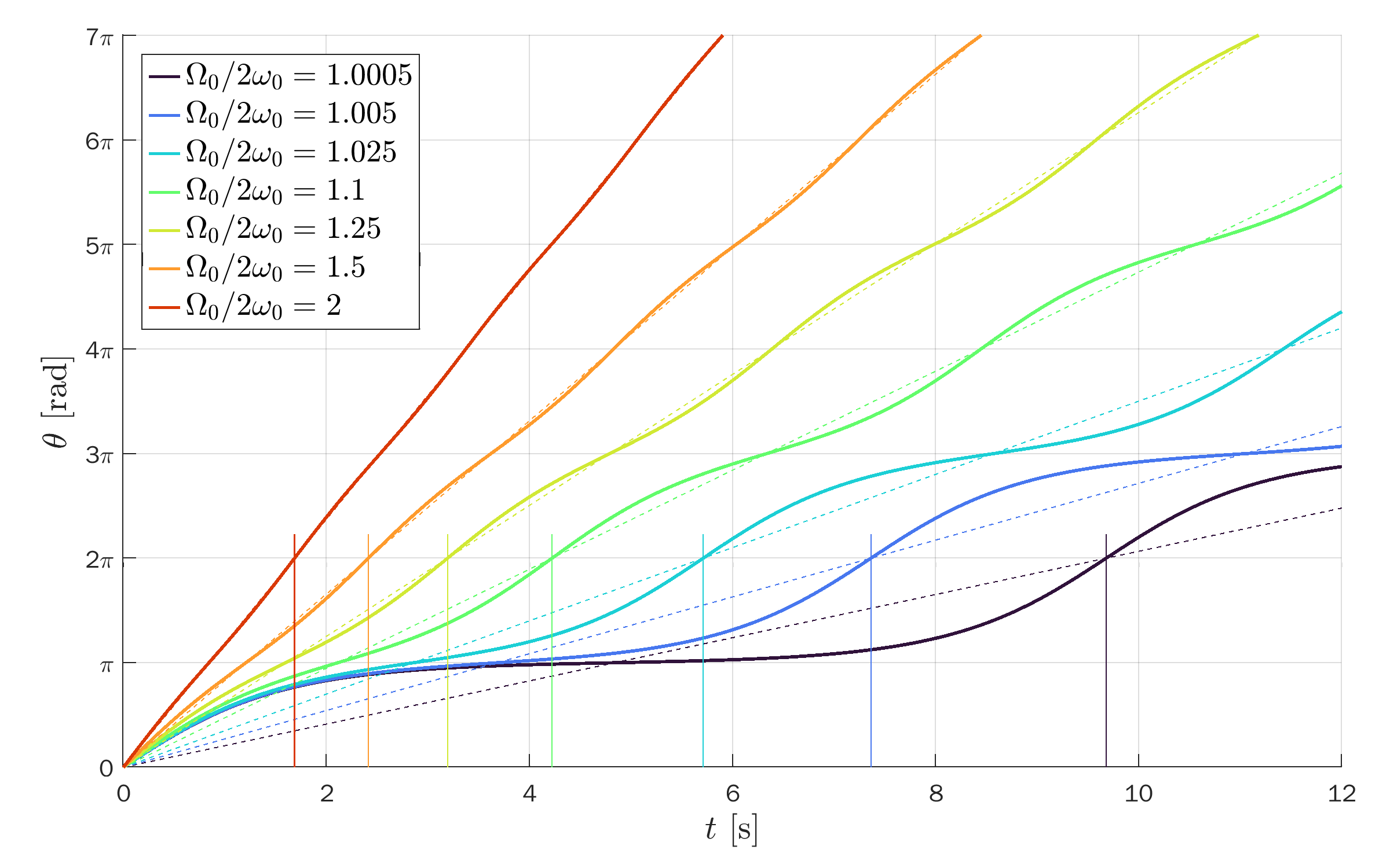
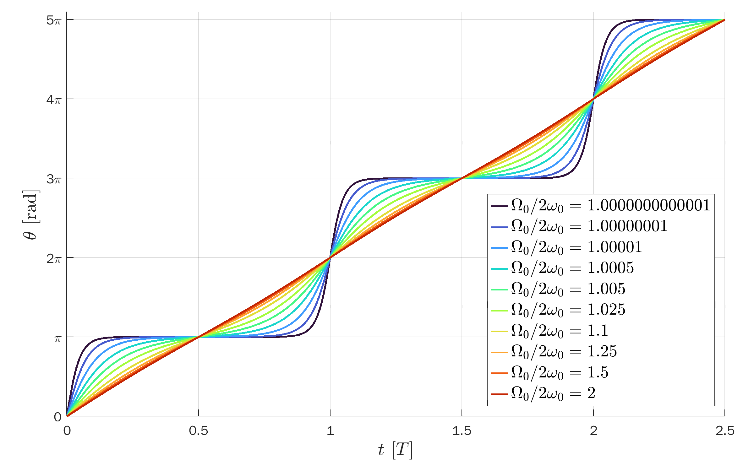
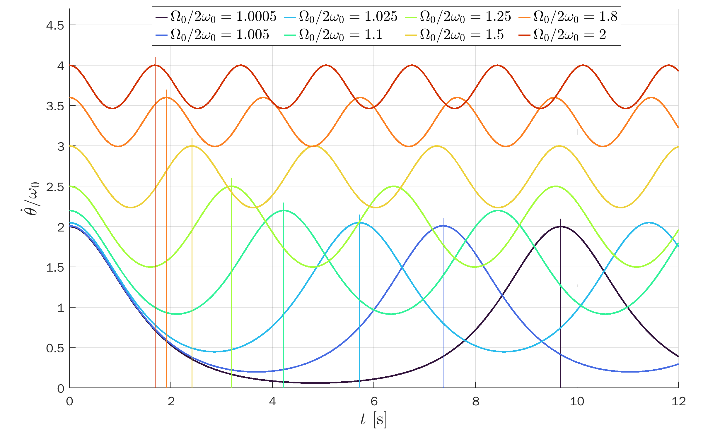
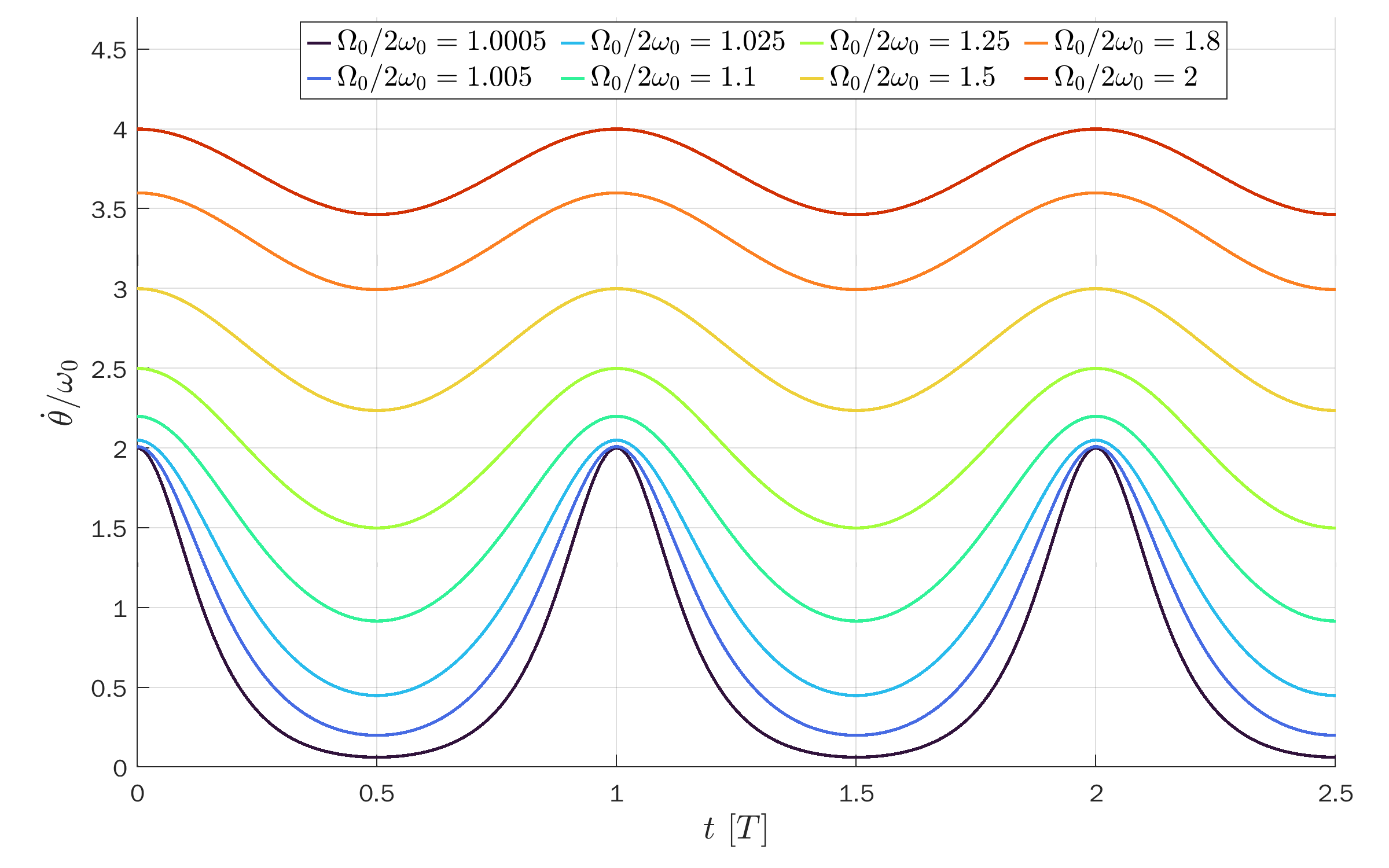
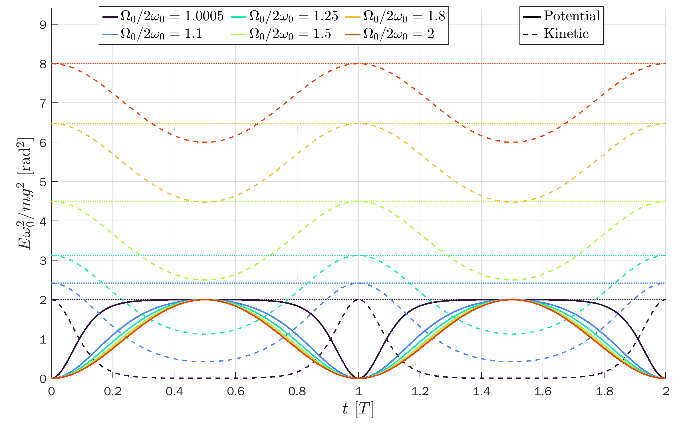
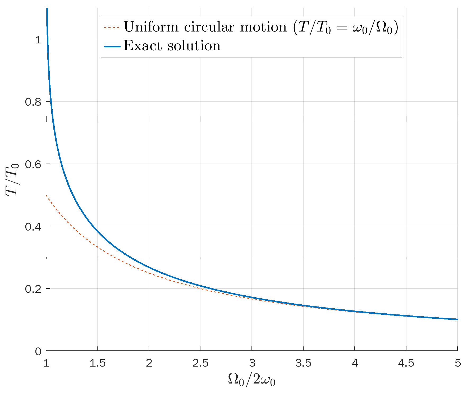
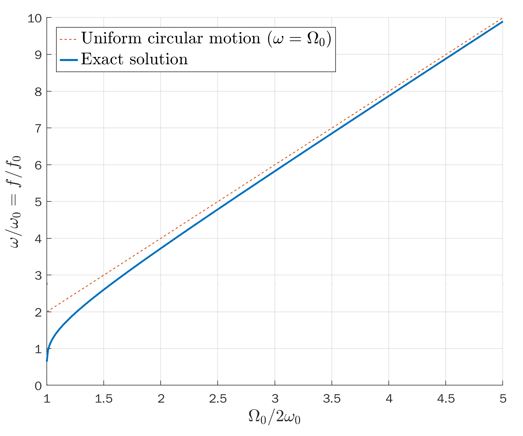
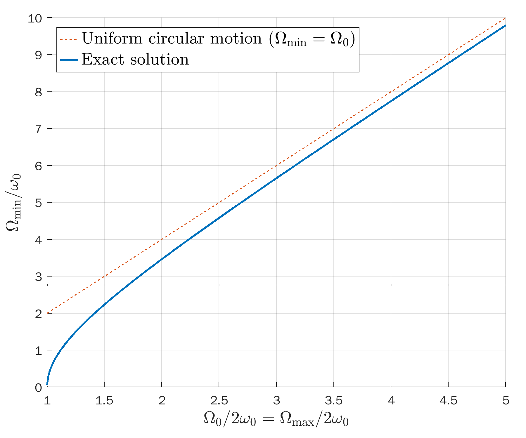
Open solutions (unbounded)
Derivation of the exact solution
Mathematical derivation of the exact solution of the pendulum with Jacobi elliptic functions (closed):
Mathematical derivation of the exact solution of the pendulum (open):
Full code
Edit and compile the full code below if you like. Note that part of the code has been disabled, because it needs to load data from external text files, which cannot be run on this website. See below for the full setup.
% Author: Izaak Neutelings (October 2020)
% Instructions: To compile, include data files from
% https://github.com/IzaakWN/CodeSnippets/tree/master/LaTeX/TikZ/physics/dynamics_pendulum
% Other sources:
% https://www.scielo.br/scielo.php?script=sci_arttext&pid=S1806-11172007000400024
% https://www.researchgate.net/publication/262746594_Exact_solution_for_the_nonlinear_pendulum
% https://tex.stackexchange.com/questions/545590/phase-portrait-of-van-der-pol-oscillator-with-pgfplots
% http://matlab.cheme.cmu.edu/2011/08/09/phase-portraits-of-a-system-of-odes/
\documentclass[border=3pt,tikz]{standalone}
\usepackage{physics}
\usepackage{siunitx}
\sisetup{detect-all} % to allow \pi in \SI
\usepackage{tikz,pgfplots}
\usepackage[outline]{contour} % glow around text
\usetikzlibrary{calc}
\usetikzlibrary{angles,quotes} % for pic
\usetikzlibrary{arrows.meta}
\tikzset{>=latex} % for LaTeX arrow head
\contourlength{1.2pt}
\colorlet{xcol}{blue!70!black}
\colorlet{vcol}{green!60!black}
\colorlet{myred}{red!70!black}
\colorlet{myblue}{blue!70!black}
\colorlet{mygreen}{green!70!black}
\colorlet{mydarkred}{myred!70!black}
\colorlet{mydarkblue}{myblue!60!black}
\colorlet{mydarkgreen}{mygreen!60!black}
\colorlet{acol}{red!50!blue!80!black!80}
\tikzstyle{CM}=[red!40!black,fill=red!80!black!80]
\tikzstyle{xline}=[xcol,thick,smooth]
\tikzstyle{mass}=[line width=0.6,red!30!black,fill=red!40!black!10,rounded corners=1,
top color=red!40!black!20,bottom color=red!40!black!10,shading angle=20]
\tikzstyle{faded mass}=[dashed,line width=0.1,red!30!black!40,fill=red!40!black!10,rounded corners=1,
top color=red!40!black!10,bottom color=red!40!black!10,shading angle=20]
\tikzstyle{rope}=[brown!70!black,very thick,line cap=round]
\def\rope#1{ \draw[black,line width=1.4] #1; \draw[rope,line width=1.1] #1; }
\tikzstyle{force}=[->,myred,very thick,line cap=round]
\tikzstyle{velocity}=[->,vcol,very thick,line cap=round]
\tikzstyle{Fproj}=[force,myred!40]
\tikzstyle{myarr}=[-{Latex[length=3,width=2]},thin]
\def\tick#1#2{\draw[thick] (#1)++(#2:0.12) --++ (#2-180:0.24)}
\DeclareMathOperator{\sn}{sn}
\DeclareMathOperator{\cn}{cn}
\DeclareMathOperator{\dn}{dn}
\def\N{80} % number of samples in plots
\begin{document}
% PENDULUM
\def\L{2.8} % string length
\def\ang{28} % angle string
\def\R{0.25} % ball radius
\def\F{1.0} % force magnitude
\begin{tikzpicture}
\message{^^JPendulum}
\coordinate (M) at (\ang-90:\L);
\coordinate (M') at (0,-\L);
\coordinate (O) at (0,0);
\coordinate (B) at (0,-\L-2.2*\R);
\coordinate (FT) at ($(M)+(90+\ang:{\F*cos(\ang)+\R})$);
\coordinate (FG) at ($(M)+(-90:{\F+\R})$);
\coordinate (FGx) at ($(M)+(-90+\ang:{0.55*\F+\R})$);
\coordinate (MA) at ($(M)+(180+\ang:{\F*sin(\ang)+\R})$);
%\draw[faded mass] (M') circle(\R);
\draw[<->] (M)++(\ang-32:0.2*\L) node[below right=-1,scale=0.9] {$x$}
--++ (\ang:0.17*\L) --++ (90+\ang:0.17*\L) node[above right=-1,scale=0.9] {$y$};
\draw[dashed] (O) -- (B);
%\draw[dashed,myred!60!black] (MA) -- (FG);
\draw[dashed,myred!60!black] (M) -- (FGx);
\draw[dashed] (-90+\ang+10:\L) arc(-90+\ang+10:-110:\L) (B);
\rope{(O) -- (M)} \path (O) -- (M) node[midway,above right=-1] {$L$};
\fill[black] (O) circle(0.04);
\draw[force] (M) -- (FT) node[midway,left=0] {$\vb{T}$};
\draw[force] (M) -- (FG) node[right=0] {$m\vb{g}$};
\draw[force,acol] (M) -- (MA) node[right=2,below=0] {$m\vb{a}$}; %{\contour{white}{$m\vb{a}$}};
\draw[mass] (M) circle(\R) node {$m$};
\draw pic[myarr,"$\theta$",xcol,draw=xcol,angle radius=22,angle eccentricity=1.30] {angle=B--O--M}; %_\text{max}
\draw pic[myarr,"$\theta$",xcol,draw=xcol,angle radius=14,angle eccentricity=1.45] {angle=FG--M--FGx};
\end{tikzpicture}
% PENDULUM FORCES - ma
\begin{tikzpicture}
\message{^^JPendulum forces}
\def\F{1.4} % force magnitude
\coordinate (O) at (0,0);
\coordinate (FT) at (90+\ang:{\F*cos(\ang)});
\coordinate (FG) at (-90:\F);
\coordinate (FGx) at (-90+\ang:{0.7*\F});
\coordinate (MA) at (180+\ang:{\F*sin(\ang)});
\draw[dashed,myred!60!black] (O) -- (FGx);
\draw[dashed,myred!60!black] (MA) -- (FG);
\draw[force] (O) -- (FT) node[midway,above right=-2] {$\vb{T}$};
\draw[force] (O) -- (FG) node[right=0] {$m\vb{g}$};
\draw[force,acol] (O) -- (MA) node[left=0] {$m\vb{a}$};
\draw pic[myarr,"$\theta$",xcol,draw=xcol,angle radius=14,angle eccentricity=1.45] {angle=FG--O--FGx};
\end{tikzpicture}
% PENDULUM FORCES
\begin{tikzpicture}
\message{^^JPendulum forces}
\def\F{1.4} % force magnitude
\coordinate (O) at (0,0);
\coordinate (FT) at (90+\ang:{\F*cos(\ang)});
\coordinate (FG) at (-90:\F);
\coordinate (FGx) at (-90+\ang:{\F*cos(\ang)});
\coordinate (FGy) at (180+\ang:{\F*sin(\ang)});
\draw[dashed,myred!60!black] (FGy) -- (FG); %-- (FGx);
\draw[force] (O) -- (FT) node[midway,above right=-2] {$\vb{T}$};
\draw[Fproj] (O) -- (FGy) node[pos=0.4,above left=-3,scale=0.86] {$mg\sin\theta$};
\draw[Fproj] (O) -- (FGx) node[pos=0.5,above right=-3,scale=0.86] {$mg\cos\theta$};
\draw[force] (O) -- (FG) node[right=0] {$m\vb{g}$};
\draw pic[myarr,"$\theta$",xcol,draw=xcol,angle radius=14,angle eccentricity=1.45] {angle=FG--O--FGx};
\end{tikzpicture}
%% PENDULUM
%\begin{tikzpicture}
% \coordinate (M) at (0,-\L);
% \coordinate (O) at (0,0);
% \rope{(O) -- (M)} \path (O) -- (M) node[midway,above right=-2] {$L$};
% \fill[black] (O) circle(0.04);
% \draw[velocity] (M)++(-\R,0) --++ (-2.7*\R,0) node[above=0] {$\vb{v}$};
% \draw[mass] (M) circle(\R) node {$m$};
%\end{tikzpicture}
% PHYSICAL PENDULUM
\begin{tikzpicture}
\message{^^JPhysical pendulum}
\def\L{2.0} % string length
\def\ang{28} % angle string
\def\R{0.25} % ball radius
\def\F{1.3} % force magnitude
\coordinate (M) at (\ang-90:\L);
\coordinate (R) at (\ang-90:1.1*\L);
\coordinate (M') at (0,-\L);
\coordinate (O) at (0,0);
\coordinate (B) at (0,-\L-2.5*\R);
\coordinate (FT) at (90:\F);
\coordinate (FG) at ($(M)+(-90:\F)$);
\coordinate (FGx) at ($(M)+(-90+\ang:{0.55*\F+\R})$);
\coordinate (MA) at ($(M)+(180+\ang:{\F*sin(\ang)+\R})$);
\draw[mass]
(180:0.3*\L) to[out=90,in=180] (80:0.36*\L) to[out=0,in=90] (0:0.3*\L) to[out=-90,in=90]
($(R)+(0:0.7*\L)$) to[out=-90,in=0] ($(R)+(-90:0.4*\L)$) to[out=180,in=-90] ($(R)+(-180:0.6*\L)$) to[out=90,in=-90] cycle; %node {$m$};
\draw[dashed] (O) -- (B);
\draw[dashed] (O) -- (M);
%\draw[dashed,myred!60!black] (MA) -- (FG);
\draw[dashed] (-90+\ang+10:\L) arc(-90+\ang+10:-110:\L) (B);
\fill[black] (O) circle(0.04);
\draw[CM] (M) circle(0.09);
\draw[force] (O) -- (FT) node[below right=0] {$\vb{F}_\mathrm{N}$};
\draw[force] (M) -- (FG) node[right=0] {$M\vb{g}$};
% \draw[force,acol] (M) -- (MA) node[right=2,below=0] {$m\vb{a}$}; %{\contour{white}{$m\vb{a}$}};
% \draw pic[myarr,"$\theta$",xcol,draw=xcol,angle radius=22,angle eccentricity=1.30] {angle=B--O--M}; %_\text{max}
% \draw pic[myarr,"$\theta$",xcol,draw=xcol,angle radius=14,angle eccentricity=1.45] {angle=FG--M--FGx};
\end{tikzpicture}
%% EXACT SOLUTION
%% Other sources:
%% https://www.scielo.br/scielo.php?script=sci_arttext&pid=S1806-11172007000400024
%% https://www.researchgate.net/publication/262746594_Exact_solution_for_the_nonlinear_pendulum
%% https://tex.stackexchange.com/questions/545590/phase-portrait-of-van-der-pol-oscillator-with-pgfplots
%% http://matlab.cheme.cmu.edu/2011/08/09/phase-portraits-of-a-system-of-odes/
%% Instructions to compile this part of the code:
%% These curves were generated numerically with these MATLAB scripts:
%% https://github.com/IzaakWN/CodeSnippets/tree/master/LaTeX/TikZ/physics/dynamics_pendulum
%% To compile this part of the code, the curves need to be loaded via external txt files.
%% To download the txt files from GitHub via the command line, do e.g.
%% wget https://github.com/IzaakWN/CodeSnippets/raw/master/LaTeX/TikZ/physics/dynamics_pendulum.zip
%% unzip dynamics_pendulum.zip
%% or
%% svn checkout https://github.com/IzaakWN/CodeSnippets/trunk/LaTeX/TikZ/physics/dynamics_pendulum/data ./dynamics_pendulum/data
%\begin{tikzpicture}
% \message{^^JPendulum exact solution}
% \def\xmax{7.0} % max x axis
% \def\ymax{1.4} % max y axis
% \def\A{3.1*\ys} % amplitude, theta0 = 3.1 ~ 178°
% \def\B{2.4*\ys} % amplitude, theta0 = 2.4 ~ 140°
% \def\C{0.6*\ys} % amplitude, theta0 = 0.6 ~ 34.4°
% \pgfmathsetmacro\Tb{\xmax/2.97} % period, theta0 = 2.4 ~ 140°, T/T0 ~ 1.5602
% \pgfmathsetmacro\Ta{\Tb*3.35/1.56} % period, theta0 = 3.1 ~ 178°, T/T0 ~ 3.3485
% \pgfmathsetmacro\Tc{\Tb*1.023/1.56} % period, theta0 = 0.6 ~ 34.4°, T/T0 ~ 1.0230
% \pgfmathsetmacro\xs{\Ta/(2*pi*3.35)} % xscale, note data uses T = 2*pi, omega0 = 1
% \pgfmathsetmacro\ys{\ymax*0.28} % yscale
%
% % AXIS
% \draw[->,thick] (0,-\ymax) -- (0,\ymax+0.2) node[above=-3] {$\theta$ [rad]};
% \draw[->,thick] (-0.2,0) -- (\xmax+0.05,0) node[right=-1] {$t$ [s]};
% \draw[mydarkblue!30,dashed]
% (0, pi*\ys) --++ (0.90*\xmax,0)
% node[right=1,scale=0.8] {$ \pi\,\si{rad}= \SI{180}{\degree}$}
% (0,-pi*\ys) --++ (0.84*\xmax,0)
% node[right=1,scale=0.8] {$-\pi\,\si{rad}=-\SI{180}{\degree}$};
%
% % PLOT REAL PENDULUM
% \begin{axis}[
% axis lines=none,anchor=origin,x=1cm,y=1cm, % coincide with TikZ coordinates
% xmin=0,xmax=0.94*\xmax/\xs,xscale=\xs,
% y filter/.code={\pgfmathparse{\ys*\pgfmathresult}}
% ]
% \addplot[xline,mygreen] table {dynamics_pendulum/data/pendulum-0p6.txt};
% \addplot[xline,myred] table {dynamics_pendulum/data/pendulum-2p4.txt};
% \addplot[xline,xcol] table {dynamics_pendulum/data/pendulum-3p1.txt};
% \end{axis}
%
% % PLOT APPROXIMATION
% \draw[xline,mydarkgreen,thin,dashed,samples=\N,smooth,variable=\x,domain=0:0.94*\xmax]
% plot(\x,{\C*cos(360/\Tc*\x)});
% \draw[xline,mydarkred,thin,dashed,samples=\N,smooth,variable=\x,domain=0:0.94*\xmax]
% plot(\x,{\B*cos(360/\Tb*\x)});
% \draw[xline,mydarkblue,thin,dashed,samples=\N,smooth,variable=\x,domain=0:0.94*\xmax]
% plot(\x,{\A*cos(360/\Ta*\x)});
%
% % TICKS
% \tick{0, \A}{0} node[above=1,left=-1,scale=0.9,mydarkblue] {3.1}; %\SI{3.1}{\degree}
% \tick{0, \B}{0} node[below=0.5,left=-1,scale=0.9,mydarkred] {2.4};
% \tick{0, \C}{0} node[below=0.5,left=-1,scale=0.9,mydarkgreen] {0.6};
% \tick{0,-\A}{0} node[left=-1,scale=0.9,mydarkblue] {$-3.1$};
% \tick{\Tb,0}{90} node[below,scale=0.9,mydarkred] {$T(2.4)$};
% \tick{2*\Tb,0}{90} node[below,scale=0.9] {$2\color{mydarkred}{T(2.4)}$};
%
%\end{tikzpicture}
%
%
%% EXACT SOLUTION - angular velocity
%\begin{tikzpicture}
% \message{^^JPendulum exact solution - dtheta/dt}
% \def\xmax{7.0} % max x axis
% \def\ymax{1.4} % max y axis
% \def\wmax{2*\ys} % yscale
% \pgfmathsetmacro\Ta{\xmax/2.97} % period, theta0 = 2.4 ~ 140°, T/T0 ~ 1.5602
% \pgfmathsetmacro\Tb{\Ta*3.35/1.56} % period, theta0 = 3.1 ~ 178°, T/T0 ~ 3.3485
% \pgfmathsetmacro\xs{\Tb/(2*pi*3.35)} % xscale, note data uses T = 2*pi, omega0 = 1
% \pgfmathsetmacro\ys{\ymax*0.44} % yscale
% \pgfmathsetmacro\A{2*sin(deg(2.4/2))*\ys} % amplitude, theta0 = 2.4 ~ 140°
% \pgfmathsetmacro\B{2*sin(deg(3.1/2))*\ys} % amplitude, theta0 = 3.1 ~ 178°
%
% % AXIS
% \draw[->,thick] (0,-\ymax) -- (0,\ymax+0.2) node[above=-3] {$\dot{\theta}$ [rad/s]};
% \draw[->,thick] (-0.2,0) -- (\xmax+0.05,0) node[right=-1] {$t$ [s]};
% \draw[mydarkblue!30,dashed]
% (0, \wmax) --++ (0.9*\xmax,0) %node[right=1,scale=0.8] {$ \SI{\pi}{rad}= \SI{180}{\degree}$}
% (0,-\wmax) --++ (0.9*\xmax,0); %node[right=1,scale=0.8] {$-\SI{\pi}{rad}=-\SI{180}{\degree}$};
%
% % PLOT REAL PENDULUM
% \begin{axis}[
% axis lines=none,anchor=origin,x=1cm,y=1cm, % coincide with TikZ coordinates
% xmin=0,xmax=0.94*\xmax/\xs,xscale=\xs,
% y filter/.code={\pgfmathparse{\ys*\pgfmathresult}}
% ]
% \addplot[xline,myred]
% table[y index=2] {dynamics_pendulum/data/pendulum-2p4.txt};
% \addplot[xline,xcol]
% table[y index=2] {dynamics_pendulum/data/pendulum-3p1.txt};
% \end{axis}
%
% % PLOT APPROXIMATION
% \draw[xline,mydarkred,thin,dashed,samples=\N,smooth,variable=\x,domain=0:0.94*\xmax]
% plot(\x,{-\A*sin(360/\Ta*\x)});
% \draw[xline,mydarkblue,thin,dashed,samples=\N,smooth,variable=\x,domain=0:0.94*\xmax]
% plot(\x,{-\B*sin(360/\Tb*\x)});
%
% % TICKS
% \tick{0, \wmax}{0} node[left=-2,scale=0.9] {$2\omega_0$};
% \tick{0,-\wmax}{0} node[left=-2,scale=0.9] {$-2\omega_0$};
% \tick{\Ta,0}{90} node[below,scale=0.9] {\contour{white}{$\color{mydarkred}{T(2.4)}$}};
% \tick{2*\Ta,0}{90} node[below,scale=0.9] {\contour{white}{$2\color{mydarkred}{T(2.4)}$}};
%
%\end{tikzpicture}
%
%
%% EXACT SOLUTION
%\begin{tikzpicture}
% \message{^^JPendulum exact solution (normalized)}
% \def\xmax{7.0} % max x axis
% \def\ymax{1.4} % max y axis
% \def\A{3.1*\ys} % amplitude, theta0 = 3.1 ~ 178°
% \def\B{2.4*\ys} % amplitude, theta0 = 2.4 ~ 140°
% \def\C{1.6*\ys} % amplitude, theta0 = 1.6 ~ 91.7
% \pgfmathsetmacro\T{0.95*\xmax/2} % period
% \pgfmathsetmacro\ys{\ymax*0.28} % yscale
%
% % AXIS
% \draw[->,thick] (0,-\ymax) -- (0,\ymax+0.2) node[above=-3] {$\theta$ [rad]};
% \draw[->,thick] (-0.2,0) -- (\xmax+0.05,0) node[right=-1] {$t$ [s]};
% \draw[mydarkblue!30,dashed]
% (0, pi*\ys) --++ (0.98*\xmax,0) node[right=1,scale=0.8] {$ \pi\,\si{rad}= \SI{180}{\degree}$}
% (0,-pi*\ys) --++ (0.90*\xmax,0) node[right=1,scale=0.8] {$-\pi\,\si{rad}=-\SI{180}{\degree}$};
%
% % PLOT REAL PENDULUM
% \begin{axis}[
% axis lines=none,anchor=origin,x=1cm,y=1cm, % coincide with TikZ coordinates
% xmin=0,xscale=\T, %0.94*7/3, %xmax=0.94*\xmax/\xs,
% y filter/.code={\pgfmathparse{\ys*\pgfmathresult}}
% ]
% \addplot[xline,mygreen] table {dynamics_pendulum/data/pendulum-1p6_norm.txt};
% \addplot[xline,myred] table {dynamics_pendulum/data/pendulum-2p4_norm.txt};
% \addplot[xline,xcol] table {dynamics_pendulum/data/pendulum-3p1_norm.txt};
% \end{axis}
%
% % PLOT APPROXIMATION
% \draw[xline,mydarkblue,thin,dashed,samples=\N,smooth,variable=\x,domain=0:0.94*\xmax]
% plot(\x,{\A*cos(360/\T*\x)});
% \draw[xline,mydarkred,thin,dashed,samples=\N,smooth,variable=\x,domain=0:0.94*\xmax]
% plot(\x,{\B*cos(360/\T*\x)});
% \draw[xline,mydarkgreen,thin,dashed,samples=\N,smooth,variable=\x,domain=0:0.94*\xmax]
% plot(\x,{\C*cos(360/\T*\x)});
%
% % TICKS
% \tick{0, \A}{0} node[above=1,left=-1,scale=0.9] {\color{mydarkblue}{3.1}};
% \tick{0, \B}{0} node[below=0.5,left=-1,scale=0.9] {\color{mydarkred}{2.4}};
% \tick{0, \C}{0} node[below=0.5,left=-1,scale=0.9] {\color{mydarkgreen}{1.6}};
% \tick{0,-\A}{0} node[left=-1,scale=0.9] {\color{mydarkblue}{$-3.1$}};
% \tick{\T,0}{90} node[below,scale=0.9] {$T$};
% \tick{2*\T,0}{90} node[below,scale=0.9] {$2T$};
%
%\end{tikzpicture}
%
%
%% EXACT SOLUTION - angular velocity
%\begin{tikzpicture}
% \message{^^JPendulum exact solution - dtheta/dt (normalized)}
% \def\xmax{7.0} % max x axis
% \def\ymax{1.4} % max y axis
% \def\wmax{2*\ys} % yscale
% \pgfmathsetmacro\T{0.95*\xmax/2} % period
% \pgfmathsetmacro\ys{\ymax*0.44} % yscale
% \pgfmathsetmacro\A{2*sin(deg(3.1/2))*\ys} % amplitude, theta0 = 3.1 ~ 178°
% \pgfmathsetmacro\B{2*sin(deg(2.4/2))*\ys} % amplitude, theta0 = 2.4 ~ 140°
% \pgfmathsetmacro\C{2*sin(deg(1.6/2))*\ys} % amplitude, theta0 = 1.6 ~ 91.7°
%
% % AXIS
% \draw[->,thick] (0,-\ymax) -- (0,\ymax+0.2) node[above=-3] {$\dot{\theta}$ [rad/s]};
% \draw[->,thick] (-0.2,0) -- (\xmax+0.05,0) node[right=-1] {$t$ [s]};
% \draw[mydarkblue!30,dashed]
% (0, \wmax) --++ (0.9*\xmax,0) %node[right=1,scale=0.8] {$ \SI{\pi}{rad}= \SI{180}{\degree}$}
% (0,-\wmax) --++ (0.9*\xmax,0); %node[right=1,scale=0.8] {$-\SI{\pi}{rad}=-\SI{180}{\degree}$};
%
% % PLOT REAL PENDULUM
% \begin{axis}[
% axis lines=none,anchor=origin,x=1cm,y=1cm, % coincide with TikZ coordinates
% xmin=0,xscale=\T,
% y filter/.code={\pgfmathparse{\ys*\pgfmathresult}}
% ]
% \addplot[xline,xcol]
% table[y index=2] {dynamics_pendulum/data/pendulum-3p1_norm.txt};
% \addplot[xline,myred]
% table[y index=2] {dynamics_pendulum/data/pendulum-2p4_norm.txt};
% \addplot[xline,mygreen]
% table[y index=2] {dynamics_pendulum/data/pendulum-1p6_norm.txt};
% \end{axis}
%
% % PLOT APPROXIMATION
% \draw[xline,mydarkblue,thin,dashed,samples=\N,smooth,variable=\x,domain=0:0.94*\xmax]
% plot(\x,{-\A*sin(360/\T*\x)});
% \draw[xline,mydarkred,thin,dashed,samples=\N,smooth,variable=\x,domain=0:0.94*\xmax]
% plot(\x,{-\B*sin(360/\T*\x)});
% \draw[xline,mydarkgreen,thin,dashed,samples=\N,smooth,variable=\x,domain=0:0.94*\xmax]
% plot(\x,{-\C*sin(360/\T*\x)});
%
% % LABELS
% \node[above=0,scale=0.8,mydarkblue] at (0.78*\T,0.99*\A) {$\theta_0=3.1$};
% \node[right,scale=0.8,mydarkred] at (0.81*\T,0.88*\B) {\contour{white}{$\theta_0=2.4$}};
% \node[right,scale=0.8,mydarkgreen] at (0.96*\T,0.4*\C) {$\theta_0=1.6$};
%
% % TICKS
% \tick{0, \wmax}{0} node[left=-2,scale=0.9] {$2\omega_0$};
% \tick{0,-\wmax}{0} node[left=-2,scale=0.9] {$-2\omega_0$};
% \tick{\T,0}{90} node[left=2,below,scale=0.9] {$T$};
% \tick{2*\T,0}{90} node[below,scale=0.9] {$2\color{mydarkred}{T}$};
%
%\end{tikzpicture}
%
%
%% EXACT SOLUTION - T/T0
%% https://en.wikipedia.org/wiki/Pendulum_(mathematics)
%\begin{tikzpicture}[xscale=1.1]
% \message{^^JPendulum exact solution period (closed/bounded)}
% \def\xmax{4.1} % max x axis
% \def\ymax{3.2} % max y axis
% \def\ys{0.82} % yscale
% \def\xs{1.02} % xscale
% \def\yz{\ys*0.4} % y zero
% \def\xtick#1{\draw[thick] (#1)++(0,0.11) --++ (0,-0.22)}
% \def\ytick#1{\draw[thick] (#1)++(0.1,0) --++ (-0.2,0)}
%
% % AXIS
% \draw[->,thick]
% (0,\yz-0.1*\ymax) -- (0,\ymax+0.1) node[below=3,left=1] {$\dfrac{T}{T_0}$};
% \draw[->,thick]
% (-0.1*\ymax,\yz) -- (\xmax,\yz) node[right=3,below=0] {$\theta_0$ [rad]};
% \draw[dashed] (\xs*pi,\yz) --++ (0,\ymax-\yz);
%
% % REAL PENDULUM
% \begin{axis}[
% axis lines=none,anchor=origin,
% x=1cm,y=1cm,ymin=0,ymax=\ymax,xscale=\xs,
% y filter/.code={\pgfmathparse{\ys*\pgfmathresult}}
% ]
% \addplot[xline]
% table[x index=0,y index=1] {dynamics_pendulum/data/pendulum_period.txt};
% \end{axis}
%
% % LINES
% \draw[dashed,mydarkgreen]
% (0,\ys) --++ (0.82*\xmax,0)
% node[right=1,scale=0.8,align=left] {small-angle\\[-1mm]approximation};
% \draw[dashed,mydarkred]
% (0,\ys*1.18) -| (0.50*pi,\yz);
%
% % TICKS
% \xtick{0.25*\xs*pi,\yz} node[below=1,scale=0.9] {$\dfrac{\pi}{4}$};
% \xtick{0.50*\xs*pi,\yz} node[below=1,scale=0.9] {$\dfrac{\pi}{2}$};
% \xtick{0.75*\xs*pi,\yz} node[below=-0.9,scale=0.9] {$\dfrac{3\pi}{4}$};
% \xtick{ \xs*pi,\yz} node[below=1,scale=0.9] {$\pi$};
% \ytick{0,\ys} node[below=1.5,left=0,scale=0.9] {1};
% \ytick{0,\ys*1.18} node[above=3,left=0,scale=0.8,mydarkred] {1.18};
% \ytick{0,\ys*2} node[left=0,scale=0.9] {2};
% \ytick{0,\ys*3} node[left=0,scale=0.9] {3};
%
%\end{tikzpicture}
%
%
%% EXACT SOLUTION - OPEN TRAJECTORY
%\begin{tikzpicture}
% \message{^^JPendulum exact solution (open/unbounded, normalized)}
% \def\xmax{7.0} % max x axis
% \def\ymax{2.8} % max y axis
% \pgfmathsetmacro\T{0.98*\xmax/2.5} % period
% \pgfmathsetmacro\ys{\ymax*0.06} % yscale
%
% % AXIS
% \draw[->,thick] (0,-0.2) -- (0,\ymax+0.2) node[above=-3] {$\theta$ [rad]};
% \draw[->,thick] (-0.2,0) -- (\xmax+0.25,0) node[right=-1] {$t$ [s]};
% \draw[mydarkblue!30,dashed,yscale=\ys]
% (0,pi) --++ (\xmax,0)
% (0,3*pi) --++ (\xmax,0)
% (0,5*pi) --++ (\xmax,0);
%
% % PLOT REAL PENDULUM
% \begin{axis}[
% axis lines=none,anchor=origin,x=1cm,y=1cm, % coincide with TikZ coordinates
% xmin=0,xscale=\T, %0.94*7/3, %xmax=0.94*\xmax/\xs,
% y filter/.code={\pgfmathparse{\ys*\pgfmathresult}}
% ]s
% \addplot[xline,xcol] table {dynamics_pendulum/data/pendulum_open-2p00000002_norm.txt};
% \addplot[xline,myred] table {dynamics_pendulum/data/pendulum_open-2p01_norm.txt};
% \addplot[xline,mygreen] table {dynamics_pendulum/data/pendulum_open-2p6_norm.txt};
% \end{axis}
%
% % LABELS
% \node[above right=-1,scale=0.8,mydarkblue] at (0.97*\T,\ys*pi) {$\Omega_0/2\omega_0=1.00000001$};
% %\node[right=2,scale=0.8,mydarkred] at (\T,1.96*\ys*pi) {\contour{white}{$\Omega_0/2\omega_0=1.005$}};
% \node[below right=0,scale=0.8,mydarkred] at (1.27*\T,3*\ys*pi) {\contour{white}{$\Omega_0/2\omega_0=1.005$}};
% %\node[below right=-1,scale=0.8,mydarkgreen] at (1.4*\T,3*\ys*pi) {$\Omega_0/2\omega_0=1.3$};
% \node[below right=0,scale=0.8,mydarkgreen] at (2.01*\T,4.24*\ys*pi) {$\Omega_0/2\omega_0=1.3$};
%
% % TICKS
% \tick{0,pi*\ys}{0} node[left=-1,scale=0.9] {$\pi$};
% \tick{0,2*pi*\ys}{0} node[left=-1,scale=0.9] {$2\pi$};
% \tick{0,3*pi*\ys}{0} node[left=-1,scale=0.9] {$3\pi$};
% \tick{0,4*pi*\ys}{0} node[left=-1,scale=0.9] {$4\pi$};
% \tick{0,5*pi*\ys}{0} node[left=-1,scale=0.9] {$5\pi$};
% \tick{\T,0}{90} node[below,scale=0.9] {$T$};
% \tick{2*\T,0}{90} node[below,scale=0.9] {$2T$};
%
%\end{tikzpicture}
%
%
%% EXACT SOLUTION - OPEN TRAJECTORIES - T/T0
%% https://en.wikipedia.org/wiki/Pendulum_(mathematics)
%\begin{tikzpicture}
% \message{^^JPendulum exact solution period (open/unbounded)}
% \def\xmax{6.1} % max x axis
% \def\ymax{2.9} % max y axis
% \def\ys{2.2} % yscale
% \def\xs{0.79} % xscale
% \def\xtick#1{\draw[thick] (#1)++(0,0.11) --++ (0,-0.22)}
% \def\ytick#1{\draw[thick] (#1)++(0.12,0) --++ (-0.24,0)}
%
% % AXIS
% \draw[->,thick] (0,-0.1*\ymax) -- (0,\ymax+0.2) node[below=3,left=1] {$\dfrac{T}{T_0}$};
% \draw[->,thick] (-0.1*\xs*\ymax,0) -- (\xs*\xmax,0) node[right=3,below=0] {$\Omega_0/2\omega_0$};
% %\draw[dashed] (pi,0) --++ (0,\ymax-0);
%
% % UNIFORM MOTION
% \draw[xline,mydarkgreen,thin,dashed,samples=\N,smooth,variable=\x,domain=\ys/(2.05*\ymax):5]
% plot(\xs*\x,{\ys/(2*\x)});
% \node[mydarkgreen,scale=0.75,above right=-4]
% at (0.12,\ymax) {uniform circular motion, $\dfrac{T}{T_0}=\dfrac{\omega_0}{\Omega_0}$};
%
% % REAL PENDULUM
% \begin{axis}[
% axis lines=none,anchor=origin,
% x=1cm,y=1cm,ymin=0,ymax=\ymax,xmin=0,xmax=5,xscale=\xs,
% y filter/.code={\pgfmathparse{\ys*\pgfmathresult}}
% ]
% \addplot[xline]
% table[x index=1,y index=2] {dynamics_pendulum/data/pendulum_period_open.txt};
% \end{axis}
%
% % LINES
% \draw[dashed,mydarkblue] (\xs,0) --++ (0,0.95*\ymax);
%
% % TICKS
% \xtick{\xs*1,0} node[below=1,scale=0.9] {$1$};
% \xtick{\xs*2,0} node[below=1,scale=0.9] {$2$};
% \xtick{\xs*3,0} node[below=1,scale=0.9] {$3$};
% \xtick{\xs*4,0} node[below=1,scale=0.9] {$4$};
% \xtick{\xs*5,0} node[below=1,scale=0.9] {$5$};
% \ytick{0,\ys*0.5} node[below=1.5,left=0,scale=0.9] {$0.5$};
% \ytick{0,\ys} node[below=1.5,left=0,scale=0.9] {$1$};
%
%\end{tikzpicture}
% PENDULUM EQUATIONS - CLOSED TRAJECTORIES
\begin{tikzpicture}[scale=1]
\message{^^JPendulum equations (closed/bounded)}
\def\myarg{\left(\alpha,k^2\right)}
\node[align=left] at (0,0) {
\begin{minipage}{9.8cm}
The differential equation for a simple pendulum is
\begin{equation*}
\dv{^2\theta}{t^2} + \omega_0^2\sin\theta = 0.
\end{equation*}
For the initial conditions
\begin{equation*}
\left\{\begin{aligned}
\theta(0) &= \theta_0\\
\left.\dv{\theta}{t}\right|_{0} &= 0
\end{aligned}\right.
\end{equation*}
with $0<\theta_0<\pi$,
the bounded solution is given by
\begin{equation*}
\theta(t)
= 2\arcsin\!\left[k\sn\!\left(\frac{\omega_0T}{4}-\omega_0t,k^2\right)\right]
\leq \theta_0,
\end{equation*}
where
\begin{equation*}
%0<\theta_0<\pi,\quad
T = \frac{4K(k^2)}{\omega_0},\quad
k = \sin{\frac{\theta_0}{2}}
\end{equation*}
and where $\sn$ is the Jacobi elliptic functions,
and $K$ is complete elliptic integral of the first kind.
The first derivative is
\begin{equation*}
\dv{\theta}{t}
= -\frac{2 k \omega_0}{\sqrt{1-(k \sn\!\myarg)^2}} \cn\!\myarg\dn\!\myarg
\end{equation*}
with $\alpha = \omega_0T/4-\omega_0t$.
%\begin{equation*}
% \alpha = \frac{\omega_0T}{4}-\omega_0t.
%\end{equation*}
The maximum angular velocity is
\begin{equation*}
\Omega_\mathrm{max} = \left.\dv{\theta}{t}\right|_{T/2} = 2k\omega_0.
\end{equation*}
Therefore, the total energy is
\begin{equation*}
E = \frac{mg^2\Omega_\mathrm{max}^2}{2\omega_0^4}
= 2\frac{mg^2}{\omega_0^2}\sin^2\frac{\theta_0}{2}.
\end{equation*}
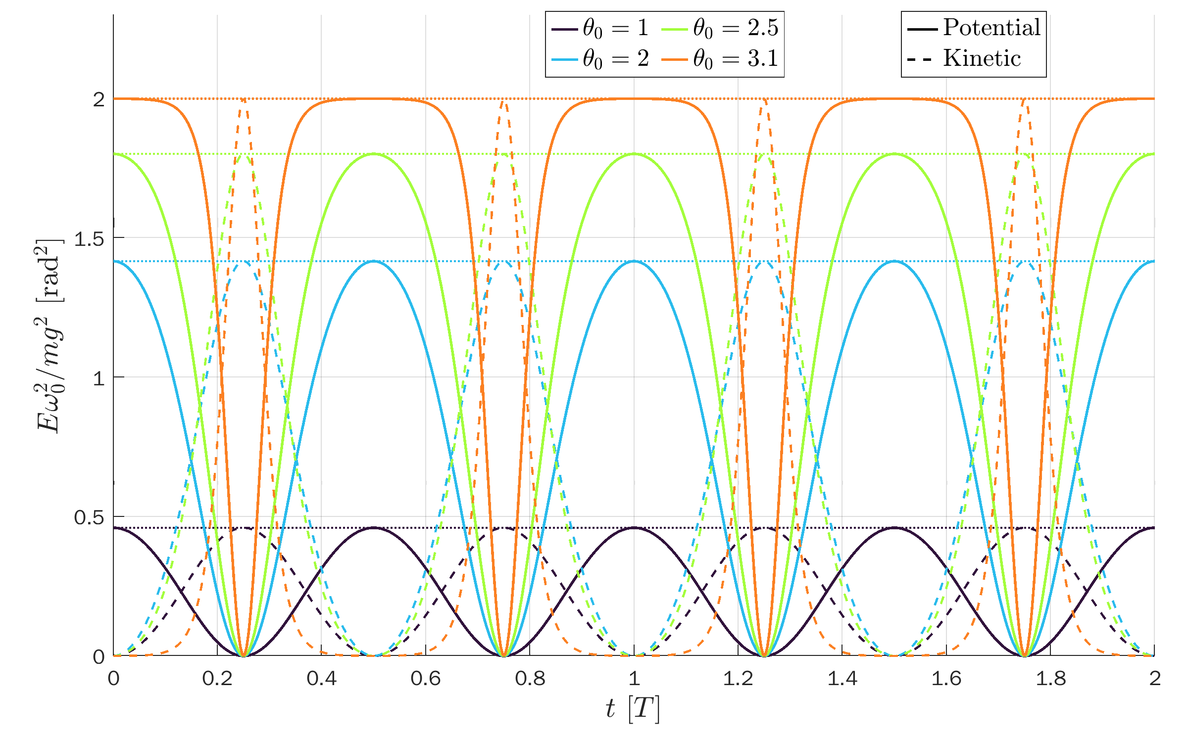
with kinetic and potential energy
\begin{align*}
K &= \frac{mg^2}{2\omega_0^4}\left(\dv{\theta}{t}\right)^2
= 2\frac{mg^2}{\omega_0^2}\left( \sin^2\frac{\theta_0}{2} - \sin^2\frac{\theta}{2} \right) \\
U &= 2\frac{mg^2}{\omega_0^2}\sin^2\frac{\theta}{2}.
\end{align*}
\end{minipage}
};
\end{tikzpicture}
% PENDULUM EQUATIONS - OPEN TRAJECTORIES
\begin{tikzpicture}[scale=1]
\message{^^JPendulum equations (open/unbounded)}
\def\myarg{\left(\frac{\Omega_0}{2}t,\frac{1}{k^2}\right)}
\node[align=left] at (0,0) {
\begin{minipage}{9.8cm}
The differential equation for a simple pendulum is
\begin{equation*}
\dv{^2\theta}{t^2} + \omega_0^2\sin\theta = 0.
\end{equation*}
For the initial conditions
\begin{equation*}
\left\{\begin{aligned}
\theta(0) &= 0 \\
\left.\dv{\theta}{t}\right|_{0} &= \Omega_0 %> 2\omega_0
\end{aligned}\right.
\end{equation*}
with $\Omega_0 > 2\omega_0$,
the unbounded solution is given by
\begin{equation*}
\theta(t)
= 2\arcsin\!\left[\sn\!\myarg\right]
\geq 0,
\end{equation*}
where
\begin{equation*}
%\Omega_0 > 2\omega_0,\quad
T = \frac{4K(k^2)}{\Omega_0},\quad
k = \frac{\Omega_0}{2\omega_0} > 2
\end{equation*}
and where sn is the Jacobi elliptic functions,
and $K$ is complete elliptic integral of the first kind.
Note that the solution $\theta(t)$ is continuous and increase monotonically,
so if one assumes $\abs{\arcsin x}\leq\pi/2$ for each real $x$,
\begin{equation*}
\theta(t)
= 2\pi n + (-1)^n 2\arcsin\!\left[\sn\!\myarg\right],
\end{equation*}
where $n=\lfloor(t+T/2)/T\rfloor=\lfloor t/T+1/2\rfloor$.\\
The first derivative is
\begin{equation*}
\dv{\theta}{t} = 2\Omega_0\dn\!\myarg,
\end{equation*}
The maximum angular velocity $\Omega_\mathrm{max}=\Omega_0$,
and the minimum is
\begin{equation*}
\Omega_\mathrm{min} = 2\omega_0\sqrt{k^2-1}.
\end{equation*}
\end{minipage}
};
\end{tikzpicture}
\end{document}
Click to download: dynamics_pendulum.zip (including input txt files) • dynamics_pendulum.tex • dynamics_pendulum.pdf
Open in Overleaf: dynamics_pendulum.zip
MATLAB figures for the exact solution of a pendulum:
Closed solutions (bounded):
Open solutions (unbounded):