Otto Cycle

Edit and compile if you like:

1
2
3
4
5
6
7
8
9
10
11
12
13
14
15
16
17
18
19
20
21
22
23
24
25
26
27
28
29
30
31
32
33
34
35
36
37
38
39
40
\documentclass[border=2pt]{standalone}
% Drawing 
\usepackage{tikz}
\usetikzlibrary{decorations.markings}
\tikzset{annotate/.style 2 args={postaction={decorate,decoration={markings,
mark=at position 0 with {\node[circle,inner sep=1.2pt,draw,fill=white,#1]{};},
mark=at position 0.52 with {\arrow[>=stealth,line width=1.5pt]{>};
\node at (0,0.4) {#2};}}}}}
% Notation
\usepackage{physics}
\usepackage{amsmath}
\begin{document}
\begin{tikzpicture}
    % P-V Axis
    \draw[latex-latex, thick] (-0.5,5) node[below left]{$P$} |- (7,0) node[below left]{$V$};
    
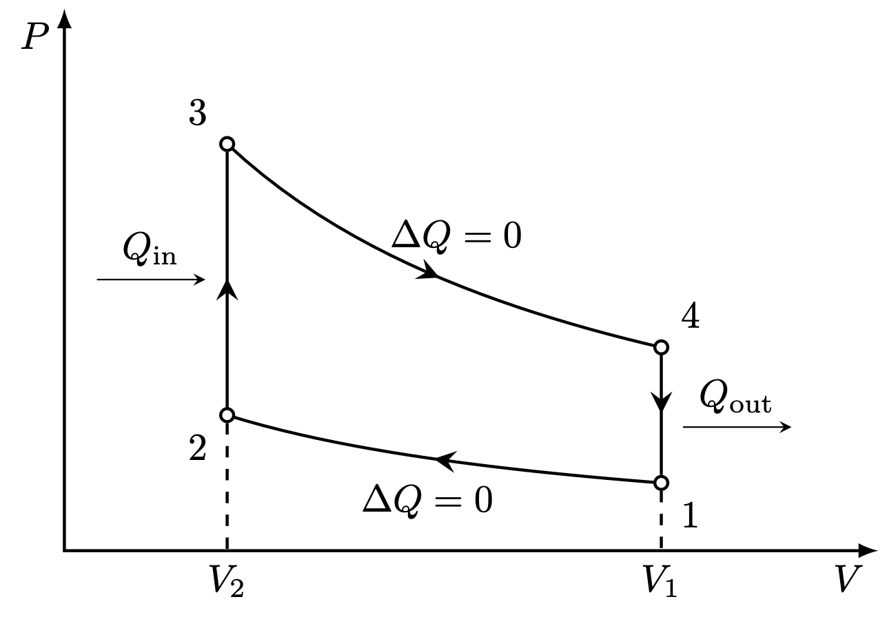
    % Otto Cycle
    \begin{scope}[thick]
    \draw[annotate={label=below right:1,alias=1}{$\Delta Q=0$}] plot[variable=\x,domain=5:1] (\x,{5/(\x+3)});
    \draw[annotate={label=above left:3,alias=3}{$\Delta Q=0$}] plot[variable=\x,domain=1:5] (\x,{15/(\x+3)});
    \draw[annotate={label=below left:2,alias=2}{}] (1,5/4) -- (3);
    \draw[annotate={label=above right:4,alias=4}{}] (5,15/8) -- (1);  
    \end{scope} 
    %
    \path (2) -- (3) coordinate[pos=0.5] (23) (1) -- (4) coordinate[pos=0.4] (14);
    
    % Q_in and Q_out
    \draw[stealth-] ([xshift=-2mm, thick]23) -- ++ (-1,0) node[midway,above]{$Q_\text{in}$};
    \draw[-stealth] ([xshift=2mm, thick]14) -- ++ (1,0) node[midway,above]{$Q_\text{out}$};
    
    % Dashed Lines  
    \draw[dashed, thick] (1) -- (1|-0,0) node[below] {$V_1$};
    \draw[dashed, thick] (2) -- (2|-0,0) node[below] {$V_2$};   
\end{tikzpicture}
\end{document}
 
 
הההההההההההההההההההההההההההההההההההההההההההההההההההההההההההההההההההההההההההההההההההההההההההההההההההההההההההההההההההההההההההההההההההההההההההההההההההההההההההההההההההההההההההההההההההההההההההההההההההההההההההההההההההההההההההההההההההההההההההההההההההההההההההההההה
XXXXXXXXXXXXXXXXXXXXXXXXXXXXXXXXXXXXXXXXXXXXXXXXXXXXXXXXXXXXXXXXXXXXXXXXXXXXXXXXXXXXXXXXXXXXXXXXXXXXXXXXXXXXXXXXXXXXXXXXXXXXXXXXXXXXXXXXXXXXXXXXXXXXXXXXXXXXXXXXXXXXXXXXXXXXXXXXXXXXXXXXXXXXXXXXXXXXXXXXXXXXXXXXXXXXXXXXXXXXXXXXXXXXXXXXXXXXXXXXXXXXXXXXXXXXXXXX