Parabolic Coordinates 3d

Edit and compile if you like:

\documentclass{article}
\usepackage{tikz}
\usepackage{tikz-3dplot}
\usetikzlibrary{math}
%\usetikzlibrary{patterns}
\usepackage[active,tightpage]{preview}
\PreviewEnvironment{tikzpicture}
\setlength\PreviewBorder{1pt}
%
% File name: Parabolic-Coordinates-3D.tex
% Description: 
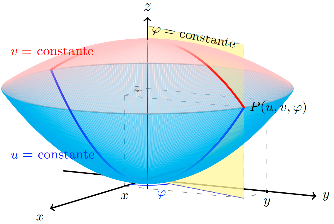
% A geometric representation of the parabolic coordinates in 3D-space is shown.
% 
% Date of creation: March,12th, 2023.
% Date of last modification: March,12th, 2023.
% Author: Efraín Soto Apolinar.
% https://www.aprendematematicas.org.mx/author/efrain-soto-apolinar/instructing-courses/
% Source: to appear in the second edition of the book titled:
% Illustrated Glossary for School Mathematics.
% https://tinyurl.com/yayyxrbz
%
% Terms of use:
% According to TikZ.net
% https://creativecommons.org/licenses/by-nc-sa/4.0/
% Your commitment to the terms of use is greatly appreciated.
%
\begin{document}
%
\tdplotsetmaincoords{80}{120}
\begin{tikzpicture}[tdplot_main_coords]
	\tikzmath{function u(\x,\y) {return abs(sqrt(sqrt(\x * \x + \y * \y) - \y)) ;};}
	\tikzmath{function v(\x,\y) {return sqrt(sqrt(\x * \x + \y * \y) + \y) ;};}
	\tikzmath{function p(\x,\y) {return atan(\y / \x) ;};}
	%
%	\tikzmath{function x(\u,\v,\p) {return \u * \v * cos(\p r);};}
%	\tikzmath{function y(\u,\v,\p) {return \u * \v * sin(\p r);};}
%	\tikzmath{function z(\u,\v,\p) {return 0.5 * (\u * \u - \v * \v);};}
	%
	\pgfmathsetmacro{\px}{1.0}
	\pgfmathsetmacro{\py}{3.0}
	\pgfmathsetmacro{\pz}{2.0}
	\pgfmathsetmacro{\angphi}{atan(\py / \px)}
	\pgfmathsetmacro{\xNode}{0.75 * cos(0.75 * \angphi)}
	\pgfmathsetmacro{\yNode}{0.75 * sin(0.75 * \angphi)}
	% Transform the coordinates of the point into parabolic coordinates
	\pgfmathsetmacro{\pu}{u(\px,\py)}
	\pgfmathsetmacro{\pv}{v(\px,\py)}
	\pgfmathsetmacro{\pp}{p(\px,\py)}
	% Domain for the graphs (u constant & v constant)
	\pgfmathsetmacro{\r}{\px * \px + \py * \py}
	% Maxima and Minima of the parabolas for u constant and v constant
	\pgfmathsetmacro{\zmaxu}{- 0.5 * \pu * \pu}
	\pgfmathsetmacro{\zmaxv}{0.5 * \pv * \pv}
	%
	\pgfmathsetmacro{\radio}{sqrt(\px * \px + \py * \py + \pz * \pz)}
	% Length of the axis
	\pgfmathsetmacro{\xaxis}{\radio + 0.5}
	\pgfmathsetmacro{\yaxis}{\radio + 0.5}
	\pgfmathsetmacro{\zaxis}{\zmaxv + 0.5}
	% Coordinate axis
	\draw[thick,->] (-0.75*\xaxis,0,0) -- (\xaxis,0,0) node [below left] {\footnotesize$x$};
	\draw[thick,->] (0,-0.5*\yaxis,0) -- (0,\yaxis,0) node [right] {\footnotesize$y$};
	\draw[thick] (0,0,\zmaxu-0.125) -- (0,0,\zmaxv); % First part of the z axis
	% Arc indicating the angle \phi
	\draw[blue] (0,0,0) -- (\px,\py,0.0);
	\draw[blue] plot[domain=0.0:\angphi,smooth,variable=\t] ({0.75 * cos(\t)},{0.75 * sin(\t)},{0.0});
	\node[blue,below] at (\xNode,\yNode) {\footnotesize$\varphi$};
	% z =  constant level curve
	\draw[gray,thick,opacity=0.75] plot[domain=0.0:2.0*pi,smooth,variable=\t] ({sqrt(\r) * cos(\t r)},{sqrt(\r) * sin(\t r)},{\pz});
	% Lines to indicate rectangular coordinates of the point P
	\draw[gray,loosely dashed] (\px,0,\pz) -- (0,0,\pz); 
	\draw[gray,loosely dashed] (0,0,\pz) -- (0,\py,\pz) -- (\px,\py,\pz);
	\draw[gray,loosely dashed] (0,\py,\pz) -- (0,\py,0) -- (\px,\py,0);
	\draw[gray,loosely dashed] (\px,0,\pz) -- (\px,0,0);
	\draw[gray,loosely dashed] (\px,\py,\pz) -- (\px,0,\pz);
	% Indications for the rectangular coordinates
	\draw[thick] (\px,0,0.025) -- (\px,0,-0.025) node [below] {\footnotesize$x$};
	\draw[thick] (0,\py,0.025) -- (0,\py,-0.025) node [below] {\footnotesize$y$};
	\draw[thick] (0,0.025,\pz) -- (0,-0.025,\pz) node [left] {\footnotesize$z$};
	% First part of the paraboloids
	\foreach \angulo in {0,1,...,180}{
		\draw[cyan,very thick,rotate around z=\angulo,opacity=0.175] (-\px,-\py,\pz) parabola bend (0,0,-0.5*\pu*\pu)(\px,\py,\pz);
	}
	\foreach \angulo in {0,1,...,180}{
		\draw[pink,very thick,rotate around z=\angulo,opacity=0.175] (-\px,-\py,\pz) parabola bend (0,0,0.5*\pv*\pv)(\px,\py,\pz);
	}
	\draw[gray,loosely dashed,fill=yellow!50,opacity=0.75] (0,0,0) parabola (\px,\py,\pz) -- (\px,\py,0.0) -- (0,0,0);	% the plane (under u = constant)
	\draw[gray,loosely dashed,fill=yellow!50,opacity=0.75] (0,0,\zmaxv) parabola (\px,\py,\pz) -- (\px,\py,\zaxis-0.2) 
		-- (0,0,\zaxis-0.2) -- (0,0,\zmaxv); % the plane (above v = constant)
	\draw[white] (\px,\py,\zaxis) -- (0,0,\zaxis) node[black,below,midway,sloped] {\footnotesize$\varphi = $ constante};
	% Parabolas obtained as trace curves with the plane \phi = constant
	\draw[blue,very thick] (-\px,-\py,\pz) parabola bend (0,0,-0.5*\pu*\pu)(\px,\py,\pz);
	\draw[red,very thick] (-\px,-\py,\pz) parabola bend (0,0,0.5*\pv*\pv)(\px,\py,\pz);
	\fill[red] (-\px,-\py,\pz) circle (0.5pt);
	% Second & last part of the paraboloids
	\foreach \angulo in {181,182,...,359}{
		\draw[cyan,very thick,rotate around z=\angulo,opacity=0.175] (-\px,-\py,\pz) parabola bend (0,0,-0.5*\pu*\pu)(\px,\py,\pz);
	}
	\draw[red,very thick] (-\px,-\py,\pz) parabola bend (0,0,0.5*\pv*\pv)(\px,\py,\pz);
	\foreach \angulo in {181,182,...,359}{
		\draw[pink,very thick,rotate around z=\angulo,opacity=0.175] (-\px,-\py,\pz) parabola bend (0,0,0.5*\pv*\pv)(\px,\py,\pz);
	}
	%
	\draw[gray,loosely dashed] (\px,0,0) -- (\px,\py,0) -- (\px,\py,\pz);	
	\node[red,above right,shift={(0,0.0,0.5)}] at (\px,-\py,\pz) {\footnotesize$v = $ constante};
	\node[blue,below right,shift={(0,0.0,-1.35)}] at (\px,-\py,\pz) {\footnotesize$u = $ constante};
	\fill[red] (\px,\py,\pz) circle (0.5pt) node[black,right] {\footnotesize$P(u,v,\varphi)$};
	\draw[thick,->] (0,0,\zmaxv) -- (0,0,\zaxis) node[above] {$z$};
	%
\end{tikzpicture}
%
\end{document}