")


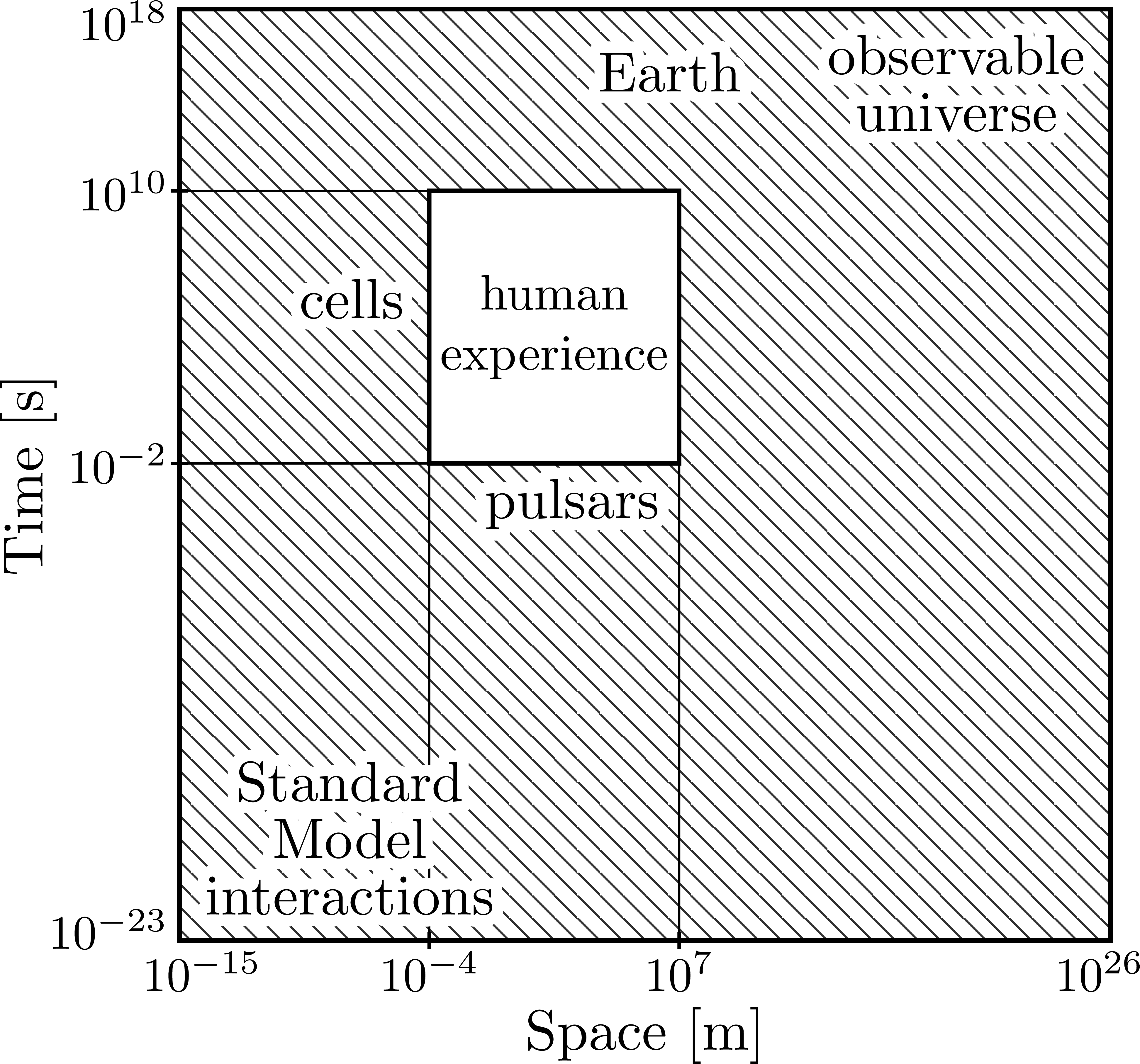
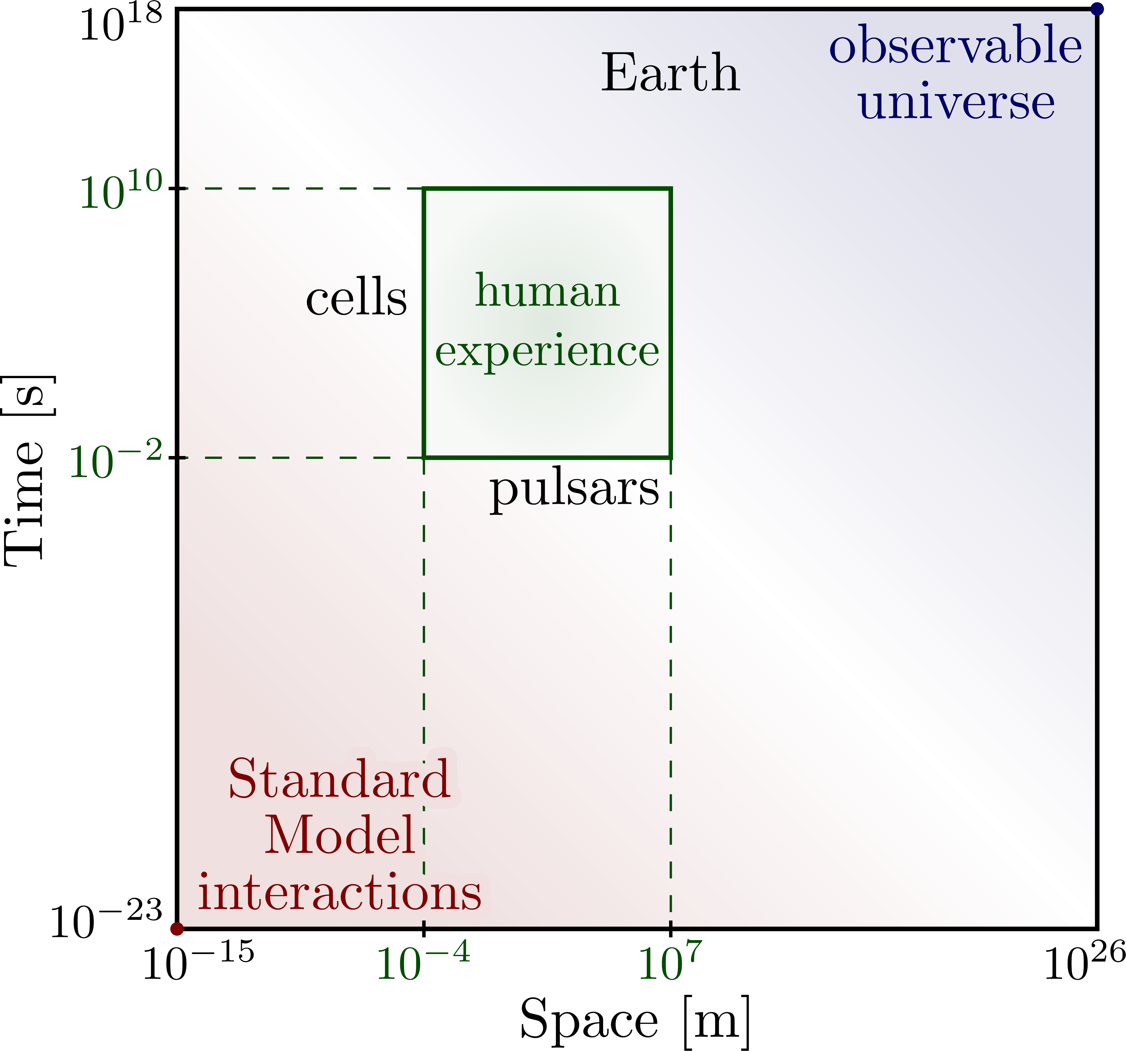
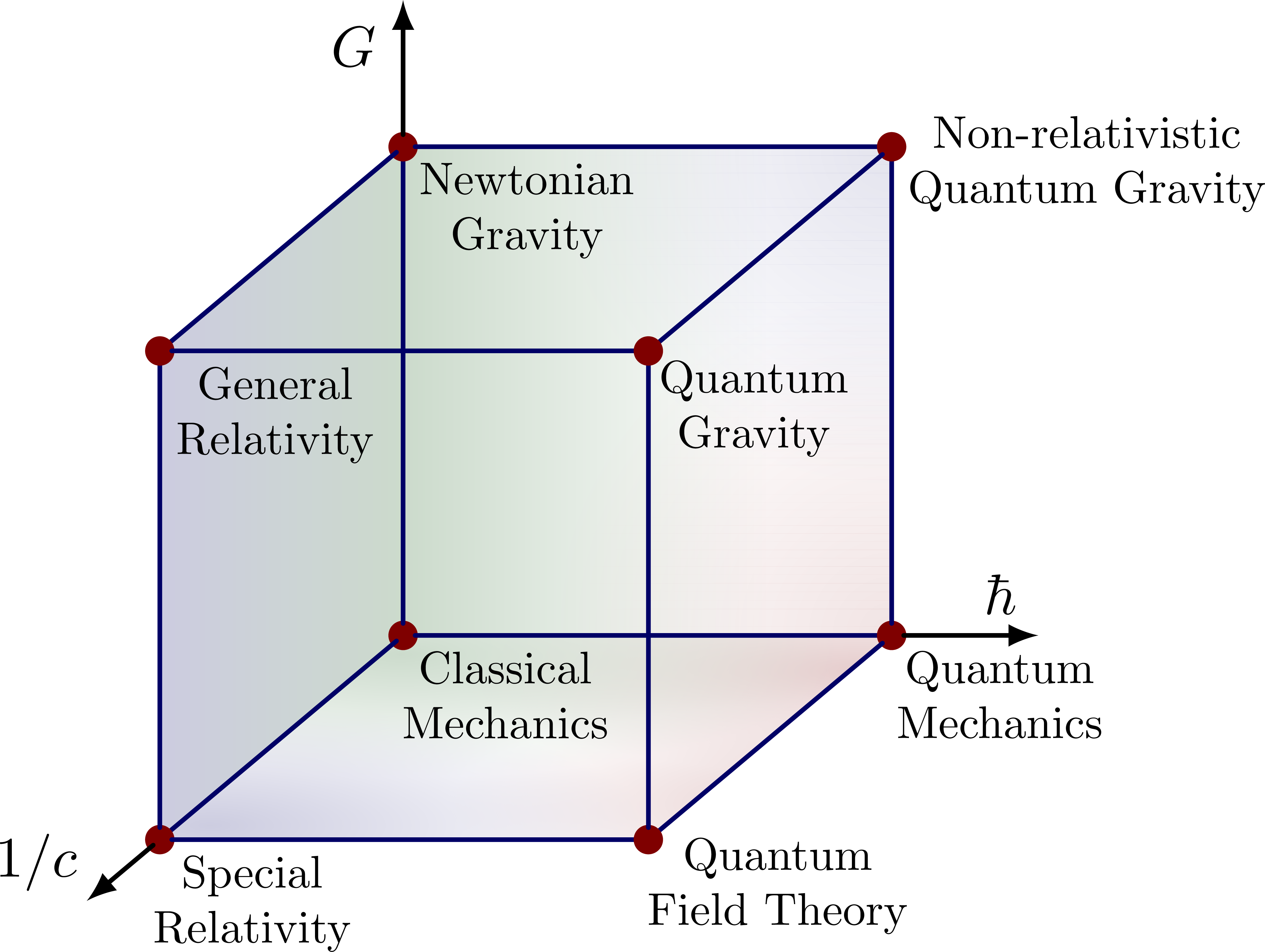
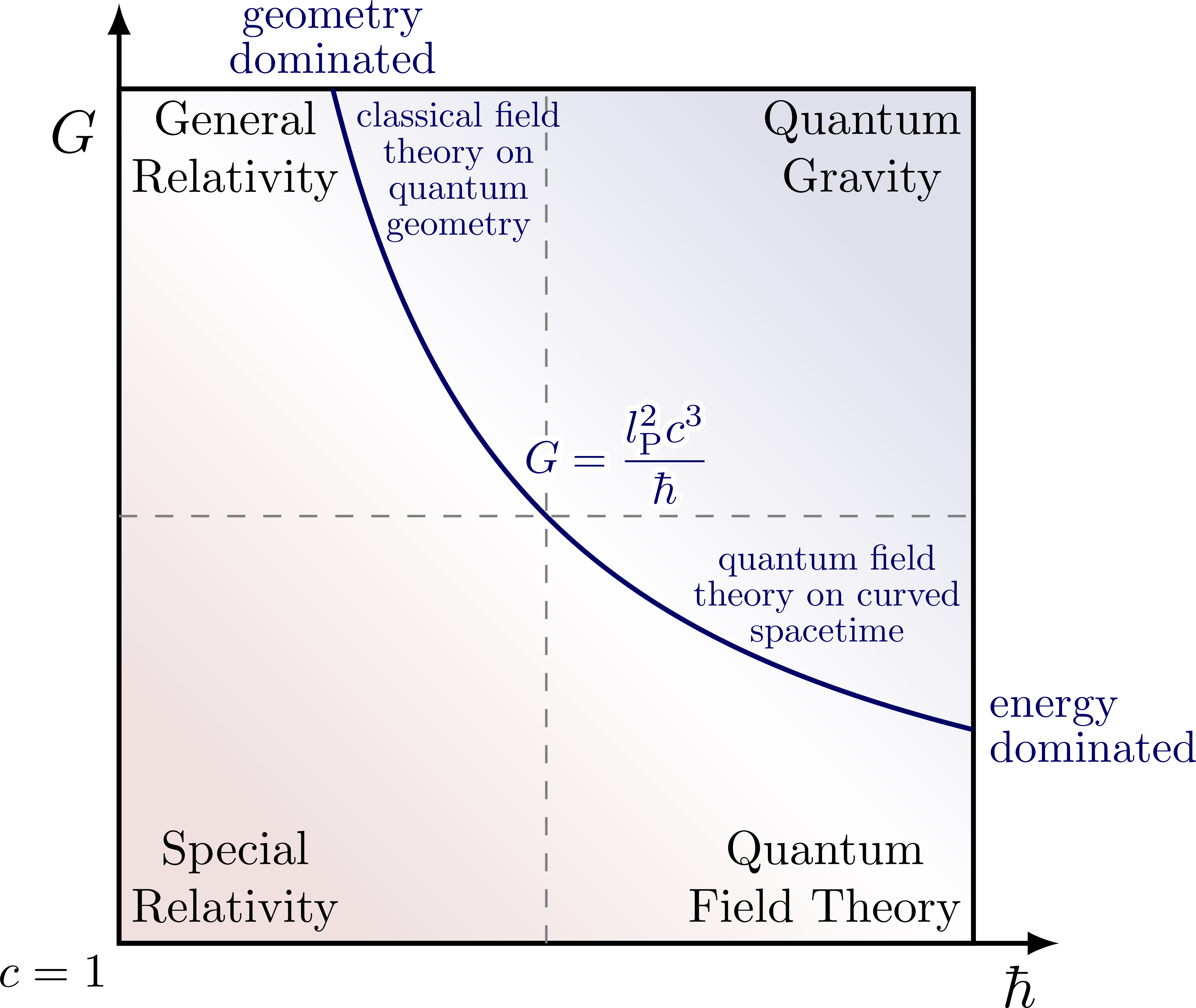
Physics domains at different spacetime scales & the Bronshtein cube (or “Bronstein cube”).
Inspired by “EUREKA!: Physics of Particles, Matter and the Universe” by R.J Blin-Stoyle.
Edit and compile if you like:
% Author: Izaak Neutelings (June 2022)
% https://pubs.aip.org/aapt/ajp/article-abstract/91/10/819/2911822/All-objects-and-some-questions?redirectedFrom=fulltext
\documentclass[border=3pt,tikz]{standalone}
\usepackage{amsmath} % for \dfrac
\usepackage{siunitx}
\usepackage[outline]{contour} % glow around text
\contourlength{1.2pt}
\usetikzlibrary{3d} % for canvas
\usetikzlibrary{shadows.blur}
\usetikzlibrary{fadings}
\usetikzlibrary{decorations.text} % for text along path
% STYLE
\tikzset{>=latex}
\tikzstyle{xlab}=[below=-1,scale=0.85]
\tikzstyle{ylab}=[left=-1,scale=0.85]
% COLORS
\colorlet{mydarkblue}{blue!40!black}
\colorlet{mylightblue}{mydarkblue!12} %blue!70!black!20
\colorlet{myred}{red!80!black}
\colorlet{mydarkred}{red!50!black}
\colorlet{mylightred}{mydarkred!12}
\colorlet{mydarkgreen}{green!30!black}
\colorlet{mylightgreen}{mydarkgreen!12}
\colorlet{myorange}{orange!63!black}
\colorlet{mylightorange}{orange!80!black!12}
% CUSTOM HATCHED (denser than default)
\usetikzlibrary{patterns} % for hatched patterns
\def\hatchsize{4pt}
\makeatletter
\pgfdeclarepatternformonly{myhatch}{%
\pgfqpoint{-1pt}{-1pt}}{\pgfqpoint{\hatchsize}{\hatchsize}}{\pgfqpoint{\hatchsize}{\hatchsize}
}{%
%\pgfsetcolor{blue!50} %\tikz@pattern@color}
\pgfsetlinewidth{0.3pt}
\pgfpathmoveto{\pgfqpoint{0pt}{\hatchsize}}
\pgfpathlineto{\pgfqpoint{\hatchsize}{0pt}}
\pgfusepath{stroke}
}
\makeatother
% CUSTOM SHADING
\tikzfading[
name=fade out,
inner color=transparent!0,
outer color=transparent!100
]
\tikzfading[
name=fade right,
left color=transparent!0,
right color=transparent!100
]
% CUSTOM SHADING
% https://tex.stackexchange.com/questions/326542/fill-a-square-with-radial-fading
\usetikzlibrary{shadings}
\makeatletter
\pgfdeclareradialshading[tikz@radial@inner,tikz@radial@outer]%
{myradial}{\pgfpointorigin}{% \pgfqpoint{-50bp}{-50bp}}{%
color(0bp)=(pgftransparent!0);%
color(20bp)=(pgftransparent!90);%
color(30bp)=(pgftransparent!93);%
color(40bp)=(pgftransparent!97);%
color(50bp)=(pgftransparent!100)%
}
%\pgfdeclareradialshading[tikz@radial@inner,tikz@radial@outer]%
% {myradial}{\pgfpointorigin}{% \pgfqpoint{-50bp}{-50bp}}{%
% color(0bp)=(tikz@radial@inner);%
% color(10bp)=(tikz@radial@outer!50!tikz@radial@inner);%
% color(25bp)=(tikz@radial@outer!60!tikz@radial@inner);%
% color(40bp)=(tikz@radial@outer!80!tikz@radial@inner);%
% color(45bp)=(tikz@radial@outer!90!tikz@radial@inner);%
% color(50bp)=(tikz@radial@outer)%
% }
%\pgfdeclareradialshading[tikz@radial@inner,tikz@radial@outer]%
% {myradial}{\pgfpointorigin}{
% color(0bp)=(tikz@radial@inner);%
% color(5bp)=(tikz@radial@outer!10!tikz@radial@inner);%
% color(20bp)=(tikz@radial@outer!90!tikz@radial@inner);%
% color(25bp)=(tikz@radial@outer)%
% }
\makeatother
%\pgfuseshading{sw radial}
\pgfdeclarefading{myradial}{\pgfuseshading{myradial}}%
\begin{document}
% SPACE & TIME SCALES
% Inspiration:
% "EUREKA!: Physics of Particles, Matter and the Universe", R.J Blin-Stoyle
% https://aniketvartak.substack.com/p/human-experience-in-a-box?r=b0a55&s=w&utm_campaign=post&utm_medium=web
\def\xmin{-15} % minimum space dimension ~ SM particles (OMG Particle: 1e-27, Planck length: 1.6e−35)
\def\xmax{ 26} % maximum space dimension ~ observable universe
\def\ymin{-23} % minimum time dimension ~ SM interactions (Planck time: 5.4e−44)
\def\ymax{18} % maximum time dimension ~ age of universe ~ 13.8 Bya = 13.8e9*365*24*3600 s
\def\xminhum{-4} % human experience xmin ~ 1e-4 m ~ 0.1 mm
\def\xmaxhum{7} % human experience xmax ~ 1e7 m ~ 12,800 km (Earth's diameter)
\def\yminhum{-2} % human experience ymin ~ 1e-2 s ~ 0.01 s
\def\ymaxhum{10} % human experience ymax ~ 3e9 s ~ 100 y = 100*365*24*3600 s
\def\tick#1#2{\draw[semithick] (#1) ++ (#2:15pt) --++ (#2-180:30pt)}
\begin{tikzpicture}[
scale=0.1,x=40,y=40,
every node/.style={align=center}, % for breaking lines in nodes
] % scale such that coordinates coincide with loglog
% HATCHED AREA
\contourlength{2pt}
\draw[thick,pattern=myhatch,pattern color=black!80]
(\xmin,\ymin) rectangle (\xmax,\ymax);
% X AXIS LABELS
\node[above,rotate=90] at ({\xmin-0.11*(\xmax-\xmin)},{(\ymin+\ymax)/2}) {Time [s]};
\node[right=4,xlab] at (\xmin,\ymin) {$10^{\xmin}$};
\node[left=2,xlab] at (\xmax,\ymin) {$10^{\xmax}$};
% Y AXIS LABELS
\node[below] at ({(\xmin+\xmax)/2},{\ymin-0.05*(\ymax-\ymin)}) {Space [m]};
\node[above=2,ylab] at (\xmin,\ymin) {$10^{\ymin}$};
\node[below=2,ylab] at (\xmin,\ymax) {$10^{\ymax}$};
% GUIDE LINES
\draw (\xminhum,\yminhum) -- (\xminhum,\ymin)
node[xlab] {$10^{\xminhum}$};
\draw (\xmaxhum,\yminhum) -- (\xmaxhum,\ymin)
node[xlab] {$10^{\xmaxhum}$};
\draw (\xminhum,\yminhum) -- (\xmin,\yminhum)
node[ylab] {$10^{\yminhum}$};
\draw (\xminhum,\ymaxhum) -- (\xmin,\ymaxhum)
node[ylab] {$10^{\ymaxhum}$};
% TICKS
\tick{\xminhum,\ymin}{90};
\tick{\xmaxhum,\ymin}{90};
\tick{\xmin,\yminhum}{0};
\tick{\xmin,\ymaxhum}{0};
% LABELS
\draw[thick,fill=white]
(\xminhum,\yminhum) rectangle (\xmaxhum,\ymaxhum)
node[midway,align=center,scale=0.88] {
human\\experience
};
\node[below left=1] at (\xmax,\ymax) {
\contour{white}{observable}\\[-2]
\contour{white}{universe}
};
\node[below] at (-7,7) { % 1d-100y = 8.640e5-3e9 s
\contour{white}{cells}
};
\node[below=4.4] at (2.7,-0.7) { % < 20 km, 1e-3-10s
\contour{white}{pulsars}
};
\node[below] at (\xmaxhum,17) { % 4.543 Bya = 1.433e17 s
\contour{white}{Earth}
};
\node[above right=1] at (\xmin,\ymin) {
\contour{white}{Standard}\\[-2]
\contour{white}{Model}\\[-2]
\contour{white}{interactions}
};
\end{tikzpicture}
% SPACE & TIME SCALES
\begin{tikzpicture}[
scale=0.1,x=40,y=40,
every node/.style={align=center}, % for breaking lines in nodes
] % scale such that coordinates coincide with loglog
% HATCHED AREA
\contourlength{2pt}
\draw[thick,left color=mylightred,right color=mylightblue,
middle color=white,shading angle=135]
(\xmin,\ymin) rectangle (\xmax,\ymax);
% X AXIS LABELS
\node[above,rotate=90] at ({\xmin-0.11*(\xmax-\xmin)},{(\ymin+\ymax)/2}) {Time [s]};
\node[right=4,xlab] at (\xmin,\ymin) {$10^{\xmin}$};
\node[left=2,xlab] at (\xmax,\ymin) {$10^{\xmax}$};
% Y AXIS LABELS
\node[below] at ({(\xmin+\xmax)/2},{\ymin-0.05*(\ymax-\ymin)}) {Space [m]};
\node[above=2,ylab] at (\xmin,\ymin) {$10^{\ymin}$};
\node[below=2,ylab] at (\xmin,\ymax) {$10^{\ymax}$};
% GUIDE LINES
\draw[dashed,mydarkgreen] (\xminhum,\yminhum) -- (\xminhum,\ymin)
node[xlab] {$10^{\xminhum}$};
\draw[dashed,mydarkgreen] (\xmaxhum,\yminhum) -- (\xmaxhum,\ymin)
node[xlab] {$10^{\xmaxhum}$};
\draw[dashed,mydarkgreen] (\xminhum,\yminhum) -- (\xmin,\yminhum)
node[ylab] {$10^{\yminhum}$};
\draw[dashed,mydarkgreen] (\xminhum,\ymaxhum) -- (\xmin,\ymaxhum)
node[ylab] {$10^{\ymaxhum}$};
% TICKS
\tick{\xminhum,\ymin}{90};
\tick{\xmaxhum,\ymin}{90};
\tick{\xmin,\yminhum}{0};
\tick{\xmin,\ymaxhum}{0};
% LABELS
\draw[thick,mydarkgreen,inner color=mylightgreen,outer color=mylightgreen!30]
(\xminhum,\yminhum) rectangle (\xmaxhum,\ymaxhum)
node[midway,align=center,scale=0.88] {
human\\experience
};
\node[mydarkblue,below left=-1] at (\xmax,\ymax) {
observable\\[-2]universe
};
\node[below] at (-7,7) {cells}; % 1d-100y = 8.640e5-3e9 s
\node[below=3] at (2.7,-0.7) {pulsars}; % < 20 km, 1e-3-10s
\node[below] at (\xmaxhum,17) {Earth}; % 4.543 Bya = 1.433e17 s
\node[mydarkred,above right=0] at (\xmin,\ymin) {
\contour{mylightred}{Standard}\\[-2]
\contour{mylightred}{Model}\\[-2]
\contour{mylightred}{interactions}
};
\fill[mydarkred] (\xmin,\ymin) circle(12pt);
\fill[mydarkblue] (\xmax,\ymax) circle(12pt);
\end{tikzpicture}
% BRONSTEIN CUBE / BRONSHTEIN CUBE
% G (Gravitation), 1/c (Velocity), hbar (Action)
% Inspiration:
% https://arxiv.org/pdf/1803.02577.pdf
% http://backreaction.blogspot.com/2011/05/cube-of-physical-theories.html
% https://www.motionmountain.net/physicscube.html
\begin{tikzpicture}[
scale=3,y={(0:1cm)},x={(-140:0.65cm)},z={(0,1cm)},
note/.style={midway,sloped,above,scale=0.5},
bar/.style={thick,blue!40!black,line cap=round},
axis/.style={->,bar,black},
point/.style={mydarkred,canvas is yz plane at x=0},
point at 1/.style={mydarkred,canvas is yz plane at x=1},
every node/.style={align=center}, % for breaking lines in nodes
]
\def\R{0.03} % sphere radius
\def\xmax{1.3}
% FILLS
\begin{scope}[canvas is xy plane at z=0]
\fill[mydarkred!20,path fading=fade out,fading transform={shift={(35:1.0)}}]
(0,-0.2) rectangle (1,1);
\fill[mydarkred!20,path fading=fade out,fading transform={shift={(-35:1.0)}}]
(0,-0.2) rectangle (1,1);
\fill[mydarkgreen!20,path fading=fade out,fading transform={shift={(112:0.8)}}]
(0,0) rectangle (1.2,1.2);
\fill[mydarkblue!20,path fading=fade out,fading transform={shift={(-135:1.1)}}]
(-0.2,0) rectangle (1,1.2);
\end{scope}
\begin{scope}[canvas is yz plane at x=0]
\clip (0,0) rectangle (1,1);
\draw[left color=mydarkgreen!20,
right color=white,middle color=white]
(0,0) rectangle (1.5,1);
\fill[path fading=fade out,mydarkred!20] (1,0) circle(0.7);
\fill[path fading=fade out,mydarkblue!20] (1,1) circle(0.7);
(0,0) rectangle (1,1);
\end{scope}
\begin{scope}[canvas is xz plane at y=0]
\clip (0,0) rectangle (1,1);
\draw[left color=mydarkblue!20,right color=mydarkgreen!20]
(0,0) rectangle (1,1);
\end{scope}
% AXES
\fill[point] (0,0) circle(\R); % (0,0,0)
\draw[bar,shorten <=50*\R] (0,0,0) -- (1,0,0);
%node[note,pos=0.50] {fast motion};
\draw[bar,shorten <=70*\R] (0,0,0) -- (0,1,0);
%node[note,pos=0.75] {tiny motion};
\draw[bar,shorten <=70*\R] (0,0,0) -- (0,0,1);
%node[note,pos=0.35,below] {bound motion};
\fill[point] (0,1) circle(\R); % (0,0,1)
\fill[point] (1,0) circle(\R); % (0,1,0)
\fill[point at 1] (0,0) circle(\R); % (1,0,0)
% EXTRA BARS
\draw[axis,shorten <=50*\R] (1,0,0) -- (\xmax,0,0) node[above left=-2] {$1/c$};
\draw[axis,shorten <=70*\R] (0,1,0) -- (0,\xmax,0) node[above left=0] {$\hbar$};
\draw[axis,shorten <=70*\R] (0,0,1) -- (0,0,\xmax) node[below left=1] {$G$};
\draw[bar,shorten <=50*\R] (0,0,1) -- (1,0,1);
\draw[bar,shorten <=70*\R] (0,0,1) -- (0,1,1);
\draw[bar,shorten <=70*\R] (1,0,0) -- (1,0,1);
\draw[bar,shorten <=70*\R] (1,0,0) -- (1,1,0);
\fill[point at 1] (0,1) circle(\R); % (1,0,1)
\draw[bar,shorten <=70*\R] (1,0,1) -- (1,1,1);
\draw[bar,shorten <=70*\R] (0,1,0) -- (0,1,1);
\draw[bar,shorten <=70*\R] (0,1,0) -- (1,1,0);
\fill[point] (1,1) circle(\R);
\draw[bar,shorten <=70*\R] (0,1,1) -- (1,1,1);
\fill[point at 1] (1,0) circle(\R);
\draw[bar,shorten <=70*\R] (1,1,0) -- (1,1,1);
\fill[point at 1] (1,1) circle(\R);
% LABELS
\node[left=3,below right,scale=0.8] at (0,0,0)
{Classical\\Mechanics};
\node[below right,scale=0.8] at (0,0,1)
{Newtonian\\Gravity};
\node[left=4,below right,scale=0.8] at (1,0,0)
{Special\\Relativity};
\node[below right,scale=0.8] at (1,0,1)
{General\\Relativity};
\node[left=2,below right=0,scale=0.8] at (0,1,0)
{Quantum\\Mechanics};
\node[below right=-3,scale=0.8] at (1,1,0)
{Quantum\\Field Theory};
\node[below=3,right,scale=0.8] at (0,1,1)
{Non-relativistic\\Quantum Gravity};
\node[below right=-1,scale=0.8] at (1,1,1)
%{Theory of\\Everything};
{Quantum\\Gravity};
\end{tikzpicture}
% Plank hyperbola (lP = sqrt(hbar*G/c^3) constant)
% https://arxiv.org/abs/2001.04491
\begin{tikzpicture}[
scale=5,
every node/.style={align=center}, % for breaking lines in nodes
]
\def\A{0.25} % hyperbola coefficient
% AXIS
\draw[thick,left color=mylightred,right color=mylightblue,
middle color=white,shading angle=135]
(0,0) rectangle (1,1);
\draw[<->,thick]
(1.1,0) node[below left=0] {$\hbar$} -|
(0,1.1) node[below left=0] at (0,1) {$G$};
\draw[black!50,dashed] (0.5,0) --+ (0,1);
\draw[black!50,dashed] (0,0.5) --+ (1,0);
% PLANCK HYPERBOLA (Planck length constant)
\draw[mydarkblue,thick,domain=\A:1,samples=100]
plot(\x,\A/\x);
\node[mydarkblue,above right=-3.5,scale=0.75] at (0.48,\A/0.48) %,rotate=-45
%{\contour{white}{$l_\mathrm{P}=\sqrt{\dfrac{\hbar G}{c^3}}$}};
{\contour{white}{$G=\dfrac{l_\mathrm{P}^2c^3}{\hbar}$}};
% REGIME LABELS
\node[scale=0.8,below left=-1] at (0,0)
{$c=1$};
\node[scale=0.8,above right=-1] at (0,0)
{Special\\Relativity};
\node[scale=0.8,above left=-1] at (1,0)
{Quantum\\Field Theory};
\node[scale=0.8,below right=-1] at (0,1)
{General\\Relativity};
\node[scale=0.8,below left=-1] at (1,1)
{Quantum\\Gravity};
% LABELS
\node[mydarkblue,scale=0.75,above=0] at (\A,1)
{geometry\\[-2]dominated};
\node[mydarkblue,scale=0.75,right=0,align=left] at (1,\A)
{energy\\[-2]dominated};
\node[mydarkblue,scale=0.6,right=3,below right=0] at (\A,1)
{classical field\\[-2] %\contour{mylightblue!70}{classical field}\\[-2]
theory on\\[-2]
quantum\\[-2]
geometry};
\node[mydarkblue,scale=0.6,above left=0] at (1,\A+0.08)
{quantum field\\[-2]
theory on curved\\[-2] spacetime};
\end{tikzpicture}
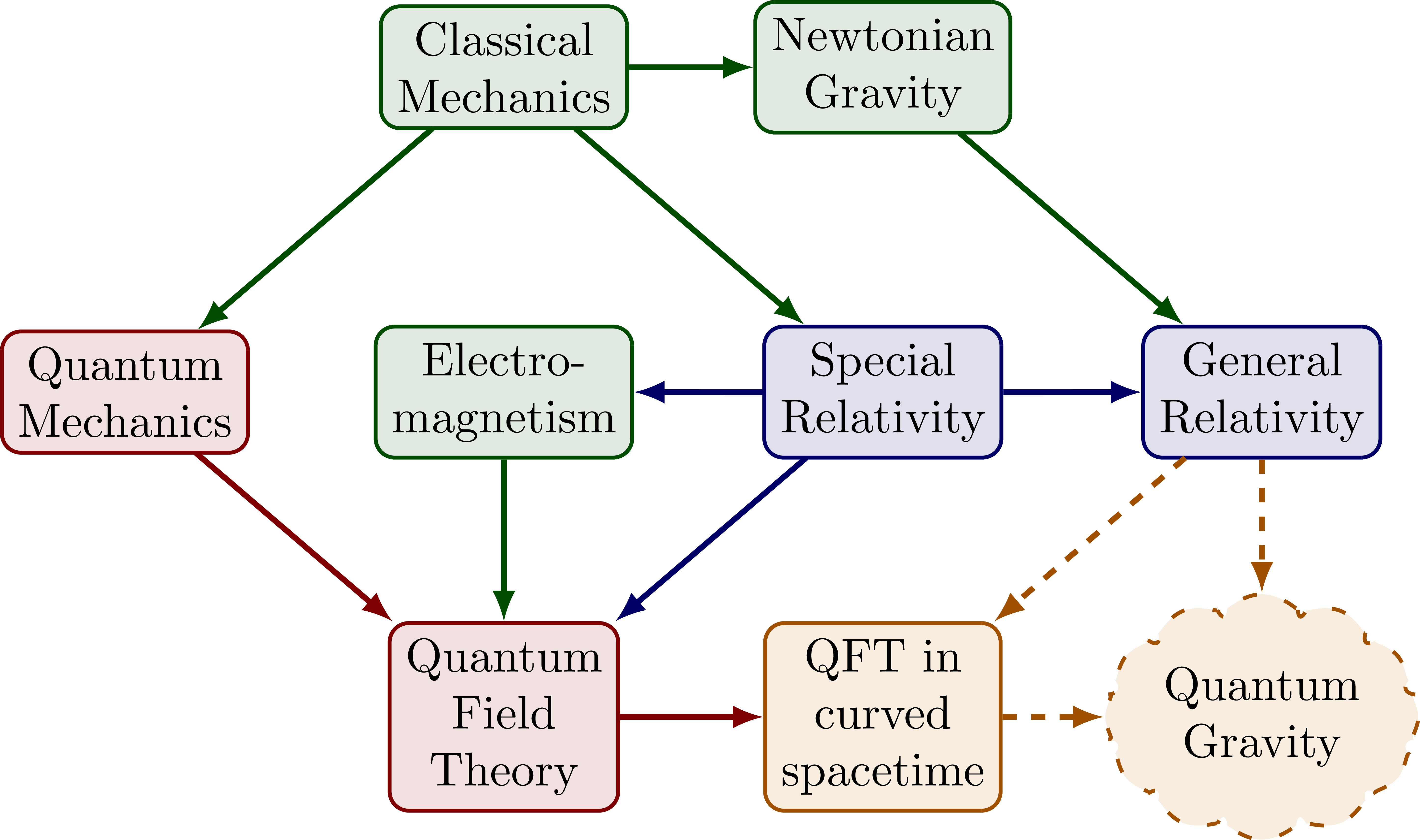
% cGh physics
% Inspiration:
% https://en.wikipedia.org/wiki/CGh_physics
\usetikzlibrary{shapes} % for cloud
\begin{tikzpicture}[
xscale=2.8,yscale=2.4,
myarrow/.style={->,very thick,draw=mydarkgreen},
myredarrow/.style={myarrow,draw=mydarkred},
mybluearrow/.style={myarrow,draw=mydarkblue},
myorangearrow/.style={myarrow,draw=myorange,dashed},
mynode/.style={thick,draw=mydarkgreen,fill=mylightgreen,rectangle,rounded corners=4,align=center},
myrednode/.style={mynode,draw=mydarkred,fill=mylightred},
mybluenode/.style={mynode,draw=mydarkblue,fill=mylightblue},
myorangenode/.style={mynode,draw=myorange,fill=mylightorange},
mycap/.style={shorten <=-0.3,line cap=round}
]
% ROW 1
\node[mynode] (CM) at (0,0) {Classical\\Mechanics};
\node[mynode] (NG) at (1,0) {Newtonian\\Gravity};
\draw[myarrow] (CM) -- (NG);
% ROW 2
\node[myrednode] (QM) at (-1,-1) {Quantum\\Mechanics};
\node[mynode] (EM) at ( 0,-1) {Electro-\\magnetism};
\node[mybluenode] (SR) at ( 1,-1) {Special\\Relativity};
\node[mybluenode] (GR) at ( 2,-1) {General\\Relativity};
\draw[mybluearrow] (SR) -- (EM);
\draw[mybluearrow] (SR) -- (GR);
% ROW 3
\node[myrednode] (QF) at (0,-2) {Quantum\\Field\\Theory};
\node[myorangenode] (CS) at (1,-2) {QFT in\\curved\\spacetime};
%\node[myrednode,dashed] (QG) at (2,-2) {Quantum\\Gravity};
\node[myorangenode,cloud,inner sep=0,loosely dashed,
aspect=1.5,cloud puffs=12,cloud puff arc=170]
(QG) at (2,-2) {Quantum\\Gravity};
\draw[myredarrow] (QF) -- (CS);
\draw[myorangearrow] (CS) -- (QG);
% ARROWS
\draw[myarrow,mycap] (CM) -- (QM);
\draw[myarrow,mycap] (CM) -- (SR);
\draw[myarrow,mycap] (NG) -- (GR);
\draw[myredarrow,mycap] (QM) -- (QF);
\draw[myarrow] (EM) -- (QF);
\draw[mybluearrow,mycap] (SR) -- (QF);
\draw[myorangearrow] (GR) -- (QG);
\draw[myorangearrow,shorten <=-0.55] (GR) -- (CS);
\end{tikzpicture}
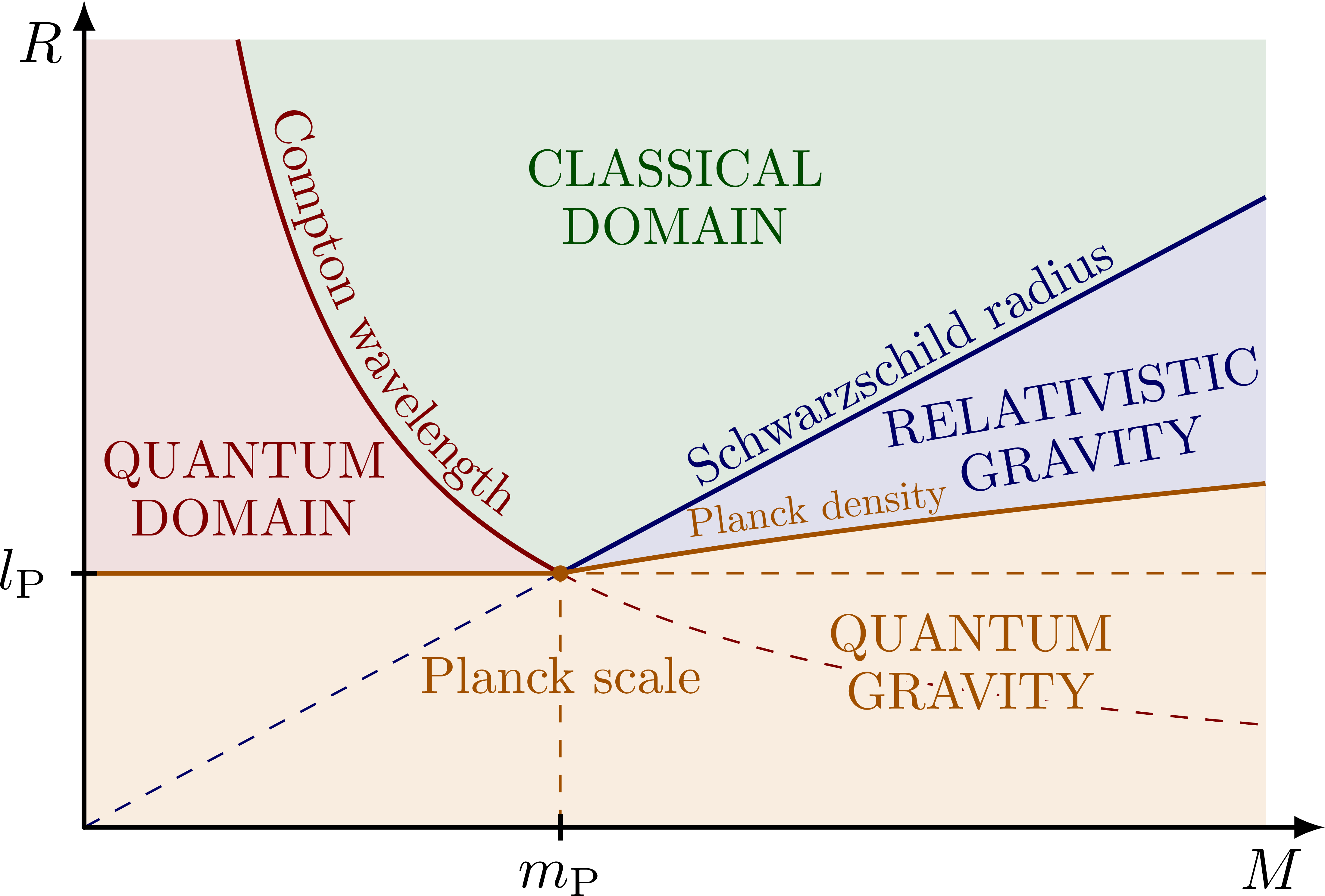
% MR-diagram
% https://arxiv.org/abs/1101.2760
\begin{tikzpicture}[
scale=4.5,x=45,y=30, % scale such that coordinates coincide with loglog
every node/.style={align=center}, % for breaking lines in nodes
]
\def\A{0.13} % hyperbola coefficient
\def\B{0.80} % slope Schwarzschild radius line
\pgfmathsetmacro\MP{sqrt(\A/\B)} % Planck mass
\pgfmathsetmacro\LP{sqrt(\A*\B)} % Planck length
\def\tick#1#2{\draw[thick] (#1) ++ (#2:0.5pt) --++ (#2-180:1pt)}
\coordinate (P) at (\MP,\LP); % Compton-Schwarschild intersection
% REGION FILLS
\fill[mylightgreen] (0,0) rectangle (1,1);
\fill[mylightorange] (0,0) rectangle (1,\LP);
\fill[mylightblue] (P) -- (1,\B) |- cycle;
\fill[mylightorange,domain=\MP:1,samples=100]
(0,0) -- (0,\LP) -- (P) plot(\x,{\LP*(\x/\MP)^(1/3)}) |- cycle;
\fill[mylightred,domain=\A:\MP,samples=100]
plot(\x,\A/\x) -| (0,1) -- cycle;
% SCHWARZSCHILD RADIUS
\draw[mydarkblue,dashed] (0,0) -- (P);
\draw[mydarkblue,thick] (P) -- (1,\B)
node[pos=0.5,sloped,above=-1.5,scale=0.9] {Schwarzschild radius};
% COMPTON WAVELENGTH HYPERBOLA
\draw[mydarkred,dashed,domain=\MP:1,samples=100]
plot(\x,\A/\x);
\draw[mydarkred,thick,domain=\A:\MP,samples=100]
plot(\x,\A/\x);
\draw[mydarkred,decorate, %postaction={decorate}
decoration={
text effects along path,
text={Compton wavelength},
text align={center},raise=3pt,
text effects/.cd,characters={text along path,scale=0.9}
},domain=\A:\MP,samples=100]
plot(\x,\A/\x);
% QUANTUM GRAVITY (Planck density): R ~ LP*(M/MP)^1/3
\draw[myorange,dashed] (\MP,0) |- (1,\LP);
%\draw[myorange,thick] (0,\LP) -- +(1,0);
\draw[myorange,thick,domain=\MP:1,samples=100]
(0,\LP) -- (P) plot(\x,{\LP*(\x/\MP)^(1/3)});
\path (P) -- (1,{\LP/\MP^(1/3)})
node[myorange,pos=0.37,sloped,above=-0.5,scale=0.7] {Planck density};
% AXIS
\draw[->,thick,line cap=round] % mass (x axis)
(0,0) -- (1.05,0)
node[below=0,below left=0] {$M$};
\draw[->,thick,line cap=round] % radius (y axis)
(0,0) -- (0,1.05)
node[below left=0] {$R$};
\tick{\MP,0}{90} node[below,scale=1] {$m_\mathrm{P}$};
\tick{0,\LP}{0} node[left,scale=1] {$l_\mathrm{P}$};
\fill[myorange] (P) circle(0.3pt);
% REGIMES LABELS
\node[mydarkgreen,scale=0.9] at (0.5,0.8)
{CLASSICAL\\[-1]DOMAIN};
\node[mydarkred,scale=0.9] at (0.135,0.43)
{QUANTUM\\[-1]DOMAIN};
\node[mydarkblue,scale=0.9,rotate=10] at (0.84,0.51)
{RELATIVISTIC\\[-1]GRAVITY};
\node[myorange,scale=0.9] at (0.75,0.21)
{QUANTUM\\[-1]\contour{mylightorange}{GRAVITY}}; %\\[-1]DOMAIN};
\node[myorange,scale=0.9] at (\MP,0.6*\LP)
{\contour{mylightorange}{Planck scale}};
\end{tikzpicture}
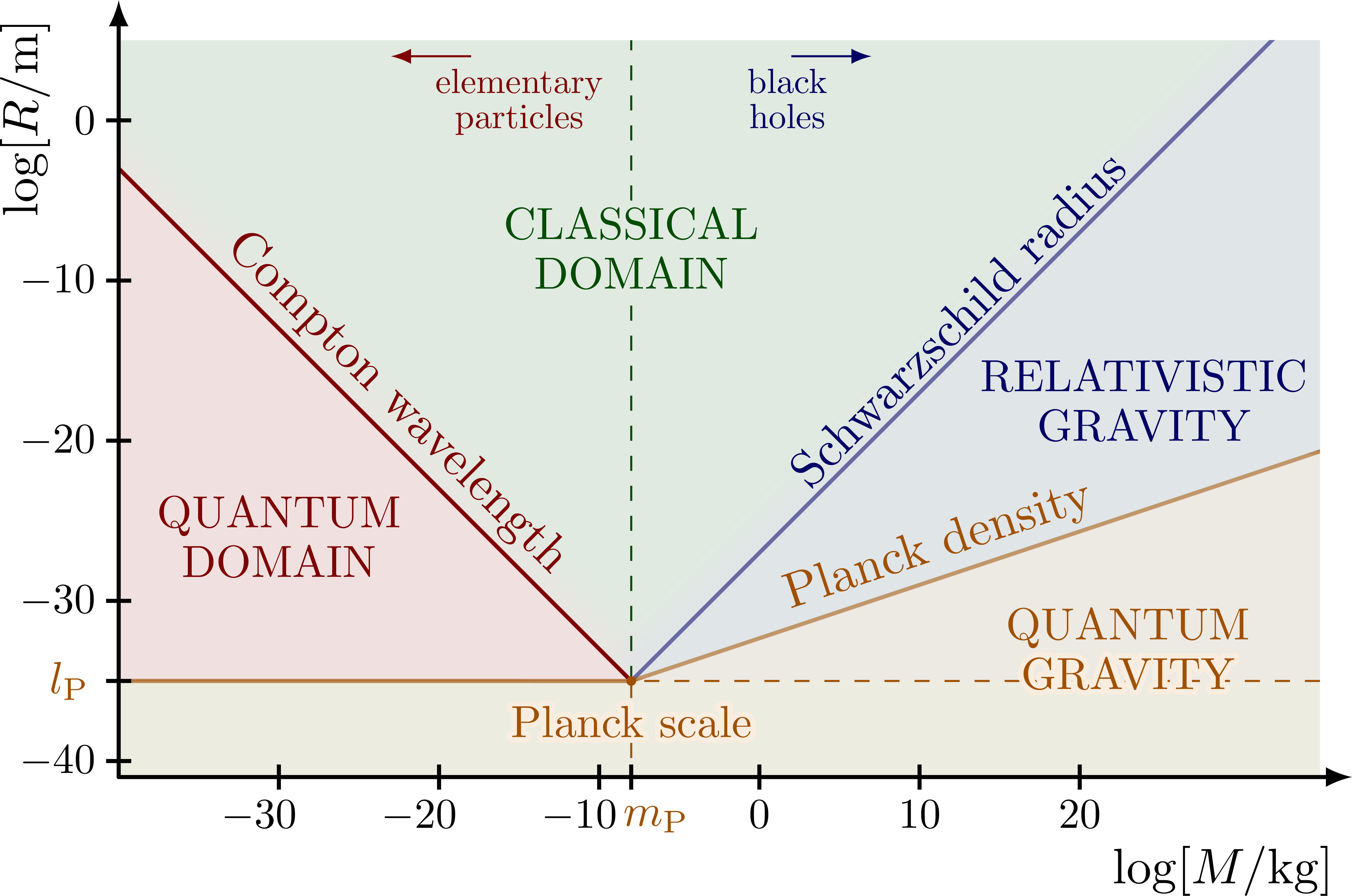
% MR-diagram (LOGLOG)
% https://arxiv.org/abs/1107.0708
% https://arxiv.org/abs/1611.01913
% Planck mass: mP = sqrt(hbar*c/G) = 2.176e-8 kg
% Planck length: lP = sqrt(hbar*G/c^3) = 1.616e-35 m
% c = 2.998e8 m/s
% G = 6.674e−11 m^3/kg/s^2
% hbar = 1.055e-34 m^2.kg/s
% hbar/c = 3.519e-43 m.kg
\begin{tikzpicture}[
scale=0.1,x=32,y=32, % scale such that coordinates coincide with loglog
every node/.style={align=center}, % for breaking lines in nodes
]
\def\xmin{-40}
\def\xmax{35}
\def\ymin{-41}
\def\ymax{5}
\def\LP{-35} % Planck length Compton-Schwarschild: sqrt(hbar*G/c^3)
\def\MP{-8} % Planck mass Compton-Schwarschild: sqrt(hbar*c/G)
\def\tick#1#2{\draw[thick] (#1) ++ (#2:25pt) --++ (#2-180:50pt)}
\coordinate (P) at (\MP,\LP); % Compton-Schwarschild intersection
\coordinate (C0) at (\xmin,{\LP+(\MP-\xmin)}); % Compton intersection with y axis
\coordinate (S0) at (\xmax,{\LP+(\xmax-\MP)}); % Schwarschild intersection with y axis
\coordinate (G0) at (\xmax,{\LP+(\xmax-\MP)/3}); % Quantum gravity intersection with y axis
\begin{scope}
\clip (\xmin,\ymin) rectangle (\xmax,\ymax);
% REGION FILLS
\fill[mylightgreen] (\xmin,\ymin) rectangle (\xmax,\ymax);
%\fill[black!20] (\xmin,\ymin) rectangle (\xmax,\LP+0.01);
\fill[mylightblue] (P) -- (S0) |- cycle;
\fill[mylightred] (P) -- (C0) |- cycle;
\fill[mylightorange] (P) -- (G0) |- (\xmin,\ymin) |- cycle;
% SHADED TRANSITION REGION
\fill[fill=mylightred,transform canvas={rotate around={45:(P)}},path fading=east]
(P) rectangle +(3,{2*(\MP-\xmin)});
\fill[fill=mylightblue,transform canvas={rotate around={-45:(P)}},path fading=west]
(P) rectangle +(-3,{2*(\xmax-\MP)});
% SCHWARZSCHILD LINE: R = 2GM/c^2 with slope 2G/c^2 = 1.485e-27 m/kg
\draw[myorange,dashed] (\xmax,\LP) -| (\MP,\ymin);
%\draw[myorange] (\MP,\ymin) -- (P);
\draw[thick,mydarkblue,line cap=round] (P) -- (S0)
node[pos=0.5,sloped,above=-2,scale=1] {Schwarzschild radius};
% QUANTUM GRAVITY (Planck density): R ~ LP*(M/MP)^1/3
\draw[thick,myorange,line cap=round] (\xmin,\LP) -- (P) -- (G0)
node[pos=0.46,sloped,above=-2,scale=1] {Planck density};
\end{scope}
% COMPTON LINE: R ~ hbar/(Mc) with slope hbar/c = 3.519e-43 m.kg
\draw[dashed,mydarkgreen] (P) -- (\MP,\ymax); % vertical divider
\draw[thick,mydarkred] (P) -- (C0)
node[pos=0.5,sloped,above=-2,scale=1] {Compton wavelength};
\fill[myorange] (P) circle(0.3);
% AXIS
\draw[->,thick,line cap=round] % log mass (x axis)
(\xmin,\ymin) -- (\xmax+2,\ymin)
node[below=10,below left=0] {$\log[M/\si{kg}]$};
\draw[->,thick,line cap=round] % log radius (y axis)
(\xmin,\ymin) -- (\xmin,\ymax+2.5)
node[left=10,above left=0,rotate=90] {$\log[R/\si{m}]$};
% TICKS
\foreach \x in {-30,-20,...,20}{
\tick{\x,\ymin}{90} node[left={\x<0?4:0},below=-1,scale=0.85] {$\x$};
}
\foreach \y in {-40,-30,-20,...,5}{
\tick{\xmin,\y}{0} node[left=-1,scale=0.85] {$\y$};
}
\tick{\MP,\ymin}{90} node[myorange,right=5,below=0,scale=0.9] {$m_\mathrm{P}$};
\tick{\xmin,\LP}{0} node[myorange,left,scale=0.9] {$l_\mathrm{P}$};
% REGIMES LABELS
\node[mydarkgreen,scale=0.9,fill=mylightgreen,inner sep=1] at (\MP,-8)
{CLASSICAL\\[-1]DOMAIN};
\node[mydarkred,scale=0.9] at (-30,-26)
{QUANTUM\\[-1]DOMAIN};
\node[mydarkblue,scale=0.9] at (24,-17.5)
{RELATIVISTIC\\[-1]GRAVITY};
\node[myorange,scale=0.9] at (23,-33)
%{QUANTUM\\[-1]GRAVITY\\[-1]\contour{mylightorange}{DOMAIN}};
{QUANTUM\\[-1]\contour{mylightorange}{GRAVITY}}; %\\[-1]DOMAIN};
\node[myorange,scale=0.9,below=2] at (P)
{\contour{mylightorange}{Planck scale}};
% LABELS
\draw[->,mydarkred] (\MP-10,\ymax-1) --++ (-5,0)
node[pos=0.6,below right,scale=0.7] {elementary\\[-2]particles};
\draw[->,mydarkblue] (\MP+10,\ymax-1) --++ (5,0)
node[pos=0.6,below left,scale=0.7] {black\\[-2]holes};
\end{tikzpicture}
\end{document}Click to download: relativity_scales.tex • relativity_scales.pdf
Open in Overleaf: relativity_scales.tex


