")


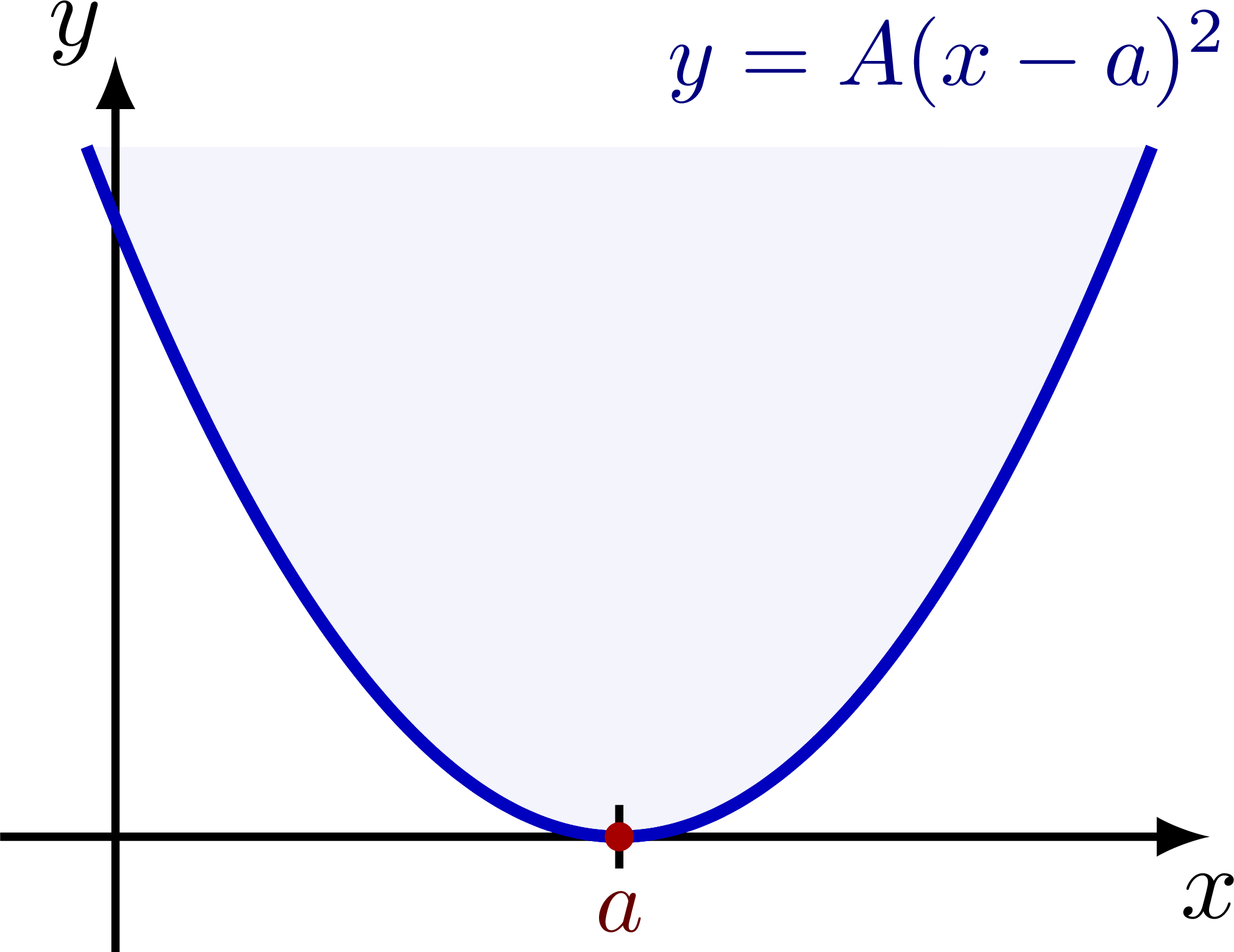
Graphical interpretation of the complex roots of a quadratic equation.
Inspired by this post and this paper.

Edit and compile if you like:
% Author: Izaak Neutelings (April 2022)
% Inspiration:
% https://math.stackexchange.com/questions/401745/help-understanding-complex-roots
% https://doi.org/10.5539/jmr.v10n6p91
\documentclass[border=3pt,tikz]{standalone}
\usepackage{amsmath}
\usepackage{tikz}
\usepackage{physics}
\usepackage[outline]{contour} % glow around text
\contourlength{1.0pt}
\usetikzlibrary{3d}
\tikzset{>=latex} % for LaTeX arrow head
\usepackage{xcolor}
\colorlet{myblue}{blue!75!black}
\colorlet{mydarkblue}{blue!50!black}
\colorlet{myred}{red!65!black}
\colorlet{mydarkred}{red!40!black}
\tikzstyle{xline}=[myblue,very thick]
\tikzstyle{round xline}=[xline,line cap=round]
\tikzstyle{area}=[xline,fill=myblue!20,fill opacity=0.5]
\tikzstyle{yzp}=[canvas is zy plane at x=0]
\tikzstyle{xzp}=[canvas is xz plane at y=0]
\tikzstyle{xyp}=[canvas is xy plane at z=0]
\def\tick#1#2{\draw[thick] (#1) ++ (#2:0.11) --++ (#2-180:0.22)}
\def\N{50}
\begin{document}
% ONE REAL solutions
\begin{tikzpicture}[scale=1]
\message{^^JReal solutions}
\def\xmin{-0.4} % x axis minimum
\def\xmax{3.8} % x axis maximum
\def\ymin{-0.4} % y axis minimum
\def\ymax{2.7} % y axis maximum
\def\tmax{1.85} % parameter t maximum (upper)
\def\A{0.7} % parabola amplitude
\def\a{1.75} % parabola minimum
\coordinate (M) at (\a,0); % parabola minimum
\coordinate (R) at (\a,0); % root
% PARABOLA BACK
\draw[area,fill opacity=0.2,samples=\N,smooth,variable=\t,domain=\a-\tmax:\a+\tmax]
plot (\t,{\A*(\t-\a)^2});
% AXES
\draw[->,black,thick] (\xmin,0) -- (\xmax,0) node[below] {$x$};
\draw[->,black,thick] (0,\ymin,0) -- (0,\ymax+0.01) node[anchor=-30,inner sep=1] {$y$};
% PARABOLA
\draw[xline,samples=\N,smooth,variable=\t,domain=\a-\tmax:\a+\tmax]
plot (\t,{\A*(\t-\a)^2});
\node[mydarkblue,left=-5,scale=0.9] at (\xmax,\ymax) {$y=A(x-a)^2$};
% TICKS
\tick{R}{90}
node[below=-1,scale=0.9,mydarkred] {$a$};
% POINTS
\fill[myred] (M) circle(0.05);
\fill[myred] (R) circle(0.05);
\end{tikzpicture}
% REAL solutions
\begin{tikzpicture}[scale=1]
\message{^^JReal solutions}
\def\xmin{-0.4} % x axis minimum
\def\xmax{3.8} % x axis maximum
\def\ymin{-0.8} % y axis minimum
\def\ymax{2.4} % y axis maximum
\def\tmax{1.85} % parameter t maximum (upper)
\def\A{0.8} % parabola amplitude
\def\a{1.75} % parabola minimum
\def\b{0.6} % parabola vertical offset
\pgfmathsetmacro\r{sqrt(\b/\A)} % root
\coordinate (M) at (\a,-\b); % parabola minimum
\coordinate (R+) at (\a+\r,0); % largest root
\coordinate (R-) at (\a-\r,0); % smallest root
% PARABOLA BACK
\draw[area,fill opacity=0.2,samples=\N,smooth,variable=\t,domain=\a-\tmax:\a+\tmax]
plot (\t,{\A*(\t-\a)^2-\b});
% AXES
\draw[->,black,thick] (\xmin,0) -- (\xmax,0) node[below] {$x$};
\draw[->,black,thick] (0,\ymin,0) -- (0,\ymax+0.01) node[anchor=-30,inner sep=1] {$y$};
% PARABOLA
\draw[xline,samples=\N,smooth,variable=\t,domain=\a-\tmax:\a+\tmax]
plot (\t,{\A*(\t-\a)^2-\b});
\node[mydarkblue,left=-5,scale=0.9] at (\xmax,\ymax) {$y=A(x-a)^2+b$};
% TICKS
\draw[mydarkred,densely dashed] (0,-\b) -- (M) -- (\a,0);
\tick{0,-\b}{0} node[left=0,scale=0.9] {$b$};
\tick{\a,0}{-90}
node[above=0,scale=0.85] {$a$};
\tick{R-}{-90}
node[left=5,above=-1,scale=0.8,mydarkred] {\contour{white}{$a-\sqrt{b/A}$}}; %\dfrac{b}{A}
\tick{R+}{-90}
node[right=7,above=-1,scale=0.8,mydarkred] {\contour{white}{$a+\sqrt{b/A}$}}; %\dfrac{b}{A}
% POINTS
\fill[myred] (M) circle(0.05);
\fill[myred] (R+) circle(0.05) (R-) circle(0.05);
\end{tikzpicture}
% IMAGINARY solutions
\def\ymax{2.7} % y axis maximum
\def\tmax{1.78} % parameter t maximum (upper)
\def\tlow{1.42} % parameter t maximum (lower)
\begin{tikzpicture}[scale=1]
\message{^^JImaginary solutions}
\def\xmin{-2.0} % x axis minimum
\def\xmax{2.2} % x axis maximum
\def\ymin{-0.8} % y axis minimum
\def\A{0.6} % parabola amplitude
\def\b{0.5} % parabola vertical offset
\pgfmathsetmacro\r{sqrt(\b/\A)} % root
\coordinate (M) at (0,\b); % parabola minimum
\coordinate (R+) at ( \r,0); % root with positive Im[z]
\coordinate (R-) at (-\r,0); % root with negative Im[z]
\coordinate (P+) at ( \r,2*\b); % root with positive Im[z], shifted
\coordinate (P-) at (-\r,2*\b); % root with negative Im[z], shifted
% PARABOLA BACK
\draw[area,fill opacity=0.2,samples=\N,smooth,variable=\t,domain=-\tmax:\tmax]
plot (\t,{\b+\A*\t*\t});
% AXES
\draw[->,black,thick] (\xmin,0) -- (\xmax,0) node[below] {$x$};
\draw[->,black,thick] (0,\ymin,0) -- (0,\ymax+0.01) node[anchor=-30,inner sep=1] {$y$};
% PARABOLA
\draw[xline,samples=\N,smooth,variable=\t,domain=-\tmax:\tmax]
plot (\t,{\b+\A*\t*\t});
\draw[area,thin,fill opacity=0.1,samples=\N,smooth,variable=\t,domain=-\tlow:\tlow]
plot (\t,{\b-\A*\t*\t});
\node[mydarkblue,right=4,scale=0.9] at (0,\ymax) {$y=Ax^2+b$};
\draw[mydarkred,densely dashed] (R+) |- (0,2*\b) -| (R-);
% TICKS
\tick{0,\b}{0} node[above=1,left=-1,scale=0.9] {\contour{white}{$b$}};
\tick{0,2*\b}{0} node[above=1,left=-1,scale=0.9] {\contour{myblue!4}{$2b$}};
\tick{-\r,0}{90}
node[left=2,below=-2,scale=0.9,mydarkred] {\contour{white}{$-\sqrt{b/A}$}}; %\dfrac{b}{A}
\tick{\r,0}{90}
node[right=2,below=-2,scale=0.9,mydarkred] {\contour{white}{$+\sqrt{b/A}$}}; %\dfrac{b}{A}
% POINTS
\fill[myred] (M) circle(0.05);
\fill[myred] (R+) circle(0.05) (R-) circle(0.05);
\fill[myred] (P+) circle(0.05) (P-) circle(0.05);
\end{tikzpicture}
% COMPLEX solutions
\begin{tikzpicture}[scale=1]
\message{^^JComplex solutions}
\def\xmin{-0.6} % x axis minimum
\def\xmax{3.5} % x axis maximum
\def\ymin{-0.3} % y axis minimum
\def\A{0.6} % parabola amplitude
\def\a{1.4} % parabola minimum
\def\b{0.5} % parabola vertical offset
\pgfmathsetmacro\r{sqrt(\b/\A)} % root
\coordinate (M) at (\a,\b); % parabola minimum
\coordinate (R+) at (\a+\r,0); % root with positive Im[z]
\coordinate (R-) at (\a-\r,0); % root with negative Im[z]
\coordinate (P+) at (\a+\r,2*\b); % root with positive Im[z], shifted
\coordinate (P-) at (\a-\r,2*\b); % root with negative Im[z], shifted
% PARABOLA BACK
\draw[area,fill opacity=0.25,samples=\N,smooth,variable=\t,domain=\a-\tmax:\a+\tmax]
plot (\t,{\b+\A*(\t-\a)^2});
% AXES
\draw[->,black,thick] (\xmin,0) -- (\xmax,0) node[below] {$x$};
\draw[->,black,thick] (0,\ymin,0) -- (0,\ymax+0.01) node[anchor=-30,inner sep=1] {$y$};
% PARABOLA
\draw[xline,samples=\N,smooth,variable=\t,domain=\a-\tmax:\a+\tmax]
plot (\t,{\b+\A*(\t-\a)^2});
\draw[area,thin,fill opacity=0.1,samples=\N,smooth,variable=\t,domain=\a-\tlow:\a+\tlow]
plot (\t,{\b-\A*(\t-\a)^2});
\node[mydarkblue,right=5,scale=0.9] at (0,\ymax) {$y=A(x-a)^2+b$};
\draw[mydarkred,densely dashed] (R+) |- (0,2*\b) -| (R-);
% TICKS
\draw[mydarkred,densely dashed] (0,\b) -- (M) -- (\a,0);
\tick{0,\b}{0} node[scale=0.9,left=-1] {$b$};
\tick{0,2*\b}{0} node[scale=0.9,left=-1] {$2b$};
\tick{\a,0}{90}
node[below=1,scale=0.8] {\contour{white}{$a$}}; %\dfrac{b}{A}
\tick{R-}{90}
node[left=5,below=-1,scale=0.8,mydarkred] {\contour{white}{$a-\sqrt{b/A}$}}; %\dfrac{b}{A}
\tick{R+}{90}
node[right=2,below=-1,scale=0.8,mydarkred] {\contour{white}{$a+\sqrt{b/A}$}}; %\dfrac{b}{A}
% POINTS
\fill[myred] (M) circle(0.05);
\fill[myred] (R+) circle(0.05) (R-) circle(0.05);
\fill[myred] (P+) circle(0.05) (P-) circle(0.05);
\end{tikzpicture}
% IMAGINARY ROOTS - extended graph
\def\xang{-10}
\def\zang{25}
\begin{tikzpicture}[y=(90:1),z=(\zang:1),x=(\xang:1),scale=1.1]
\message{^^JImaginary solutions - extended graph}
\def\xmax{1.8} % x axis maximum
\def\ymin{-1.3} % y axis minimum
\def\ymax{2.7} % y axis maximum
\def\zmax{1.8} % z axis maximum
\def\tmax{1.0} % parameter t maximum (upper)
\def\tlow{1.1} % parameter t maximum (lower)
\def\A{1.5} % parabola amplitude
\def\b{0.95} % parabola vertical offset
\pgfmathsetmacro\r{sqrt(\b/\A)} % root
\coordinate (M) at (0,\b,0); % parabola minimum
\coordinate (R+) at (0,0, \r); % root with positive Im[z]
\coordinate (R-) at (0,0,-\r); % root with negative Im[z]
% AXES
\draw[black,thick] (-\xmax,0,0) -- (0,0,0);
% PARABOLA
\draw[area,samples=\N,smooth,variable=\t,domain=-\tlow:\tlow]
plot (0,{\b-\A*\t*\t},\t);
\draw[area,samples=\N,smooth,variable=\t,domain=-\tmax:\tmax]
plot (\t,{\A*\t*\t+\b},0);
\node[mydarkblue,right=7,scale=0.9] at (0,0.96*\ymax,0) {$y=Ax^2+b$};
\node[mydarkblue,below=5,left=4,scale=0.9] at (0,\ymin,0) {$y=b-At^2$};
% AXES
\draw[->,black,thick] (0,\ymin,0,0) -- (0,\ymax+0.06,0) node[above left=-3] {$y$};
\draw[->,black,thick] (0,0,-\zmax) -- (0,0,\zmax) node[right=8,above=-2] {$t=\Im[z]$};
% POINTS
\tick{0,\b,0}{0} node[left=1] {$b$};
\fill[myred] (M) circle(0.05);
\fill[myred,xzp]
(R+) circle(0.05)
(R-) circle(0.05);
% FRONT
\draw[round xline,samples=\N,smooth,variable=\t]
plot[domain=0.006-\r:-0.01] (0,{\b-\A*\t*\t},\t)
plot[domain=\r/2:\r-0.008] (0,{\b-\A*\t*\t},\t);
\draw[->,black,thick,line cap=round]
(0.01,0,0) -- (\xmax,0,0) node[right=5,below=0] {$x=\Re[z]$};
% TICKS
\tick{R-}{-90} node[mydarkred,scale=0.9,anchor=-5,inner sep=2] {$-\sqrt{b/A}$};
\tick{R+}{90} node[mydarkred,scale=0.9,anchor=186,inner sep=2] {$+\sqrt{b/A}$};
\end{tikzpicture}
% COMPLEX ROOTS - extended graph
\def\xang{-7}
\def\zang{25}
\begin{tikzpicture}[y=(90:1),z=(\zang:1),x=(\xang:1),scale=1.2]
\message{^^JComplex solutions - extended graph}
\def\xmax{3.2} % x axis maximum
\def\ymin{-1.3} % y axis minimum
\def\ymax{2.8} % y axis maximum
\def\zmin{-1.6} % z axis minimum
\def\zmax{2.4} % z axis maximum
\def\tmax{1.00} % parameter t maximum (upper)
\def\tlow{1.10} % parameter t maximum (lower)
\def\A{1.5} % parabola amplitude
\def\a{1.5} % parabola minimum
\def\b{1.1} % parabola vertical offset
\pgfmathsetmacro\r{sqrt(\b/\A)} % root
\coordinate (M) at (\a,\b,0); % parabola minimum
\coordinate (R+) at (\a,0, \r); % root with positive Im[z]
\coordinate (R-) at (\a,0,-\r); % root with negative Im[z]
% AXES
\draw[black,thick] (-0.1*\ymax,0,0) -- (\a,0,0);
\draw[->,black,thick] (0,\ymin,0,0) -- (0,\ymax,0) node[above left=-3] {$y$};
\draw[->,black,thick] (0,0,\zmin) -- (0,0,\zmax) node[above=1,right=1] {$t=\Im[z]$};
\draw[mydarkred,densely dashed]
(R+) -- (0,0,\r);
% PARABOLA
\draw[area,samples=\N,smooth,variable=\t,domain=-\tlow:\tlow]
plot (\a,{\b-\A*\t*\t},\t);
\draw[area,samples=\N,smooth,variable=\t,domain=\a-\tmax:\a+\tmax]
plot (\t,{\b+\A*(\t-\a)^2},0);
\node[mydarkblue,right=2,scale=0.9] at (\a,\ymax,0) {$y=A(x-a)^2+b$};
\node[mydarkblue,right=0,scale=0.9] at (0.6*\a,0.9*\ymin,0) {$y=b-At^2$ ($x=a$)};
% POINTS
\fill[myred] (M) circle(0.05);
\fill[myred,xzp]
(R+) circle(0.05)
(R-) circle(0.05);
\draw[mydarkred,densely dashed]
(M) -- (0,\b,0)
(R-) -- (0,0,-\r)
(R+) -- (R-);
% FRONT
\draw[round xline,samples=\N,smooth,variable=\t]
plot[domain=0.006-\r:-0.01] (\a,{\b-\A*\t*\t},\t)
plot[domain=\r/2:\r-0.008] (\a,{\b-\A*\t*\t},\t);
\draw[->,black,thick,line cap=round]
(\a,0,0) -- (\xmax,0,0) node[right=5,below=0] {$x=\Re[z]$};
% TICKS
\tick{\a,0,0}{90} node[below=-1] {$a$};
\tick{0,0,-\r}{-90}
node[mydarkred,scale=0.9,anchor=-40,inner sep=0] {$-\sqrt{b/A}$};
\tick{0,0,\r}{-90}
node[mydarkred,scale=0.9,anchor=-40,inner sep=0] {$+\sqrt{b/A}$};
\tick{0,\b,0}{0} node[left=0] {$b$};
\end{tikzpicture}
% QUADRATIC EQUATION
\begin{tikzpicture}[scale=1]
\node[align=left] at (0,0) {
\begin{minipage}{9.2cm}
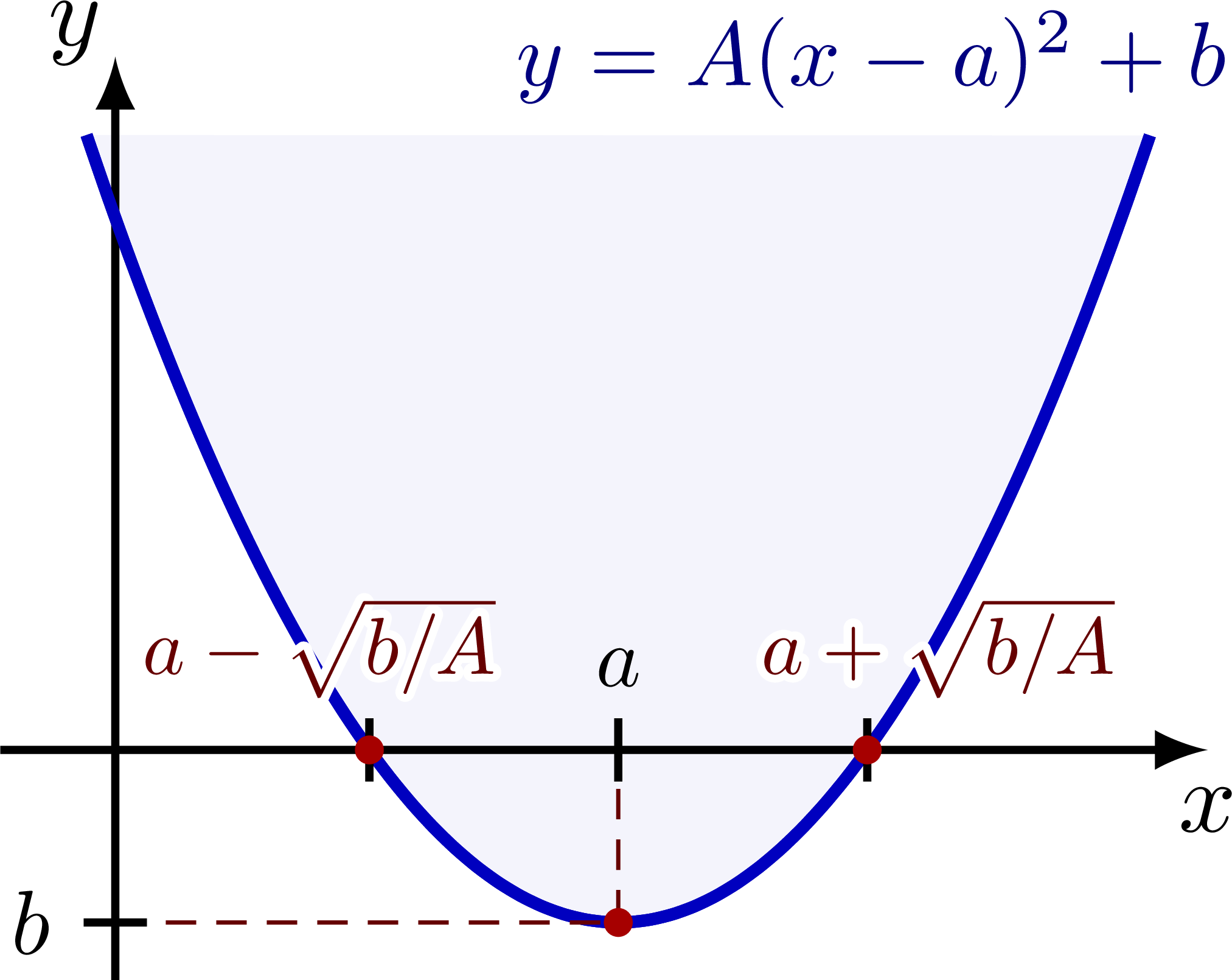
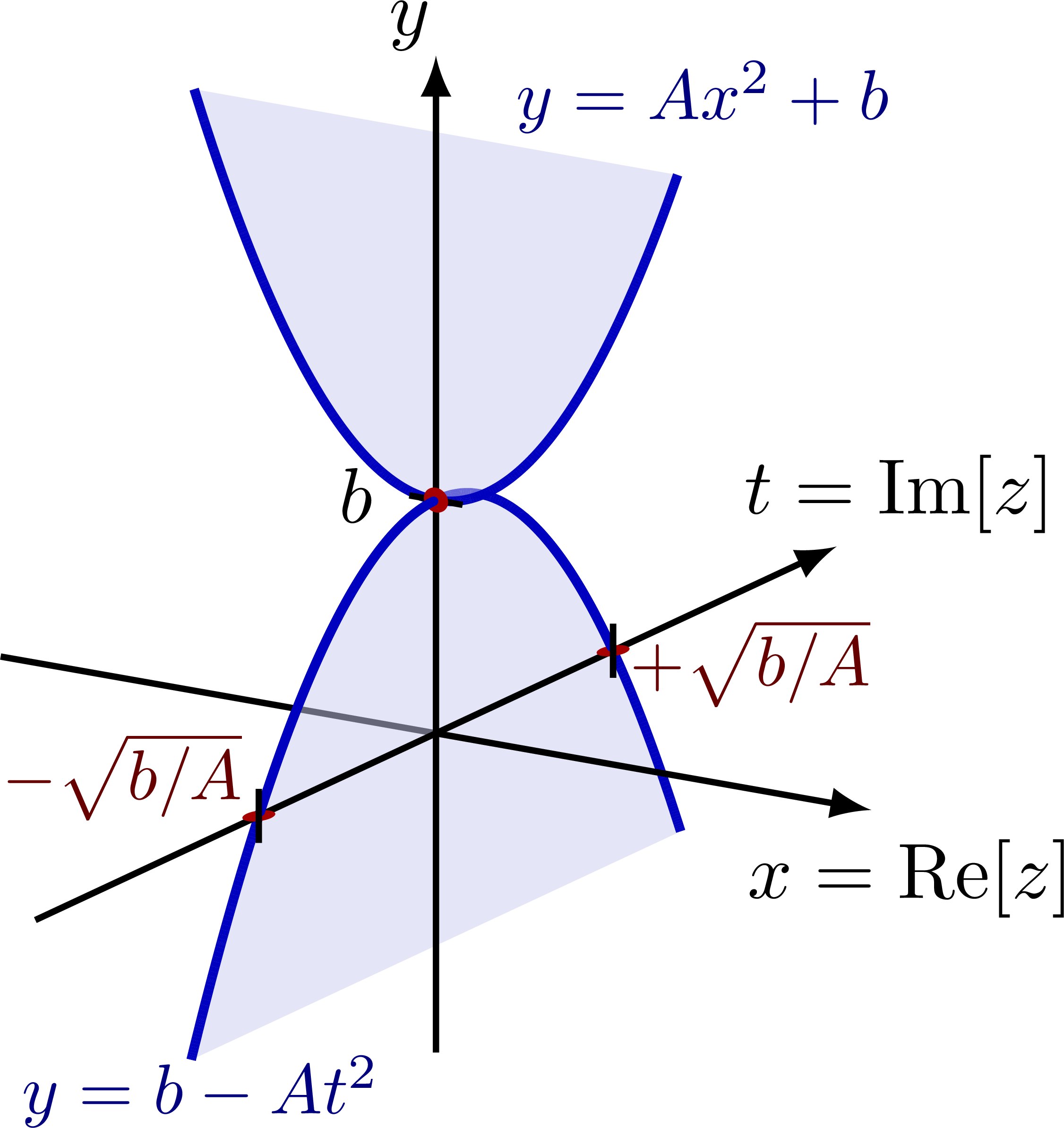
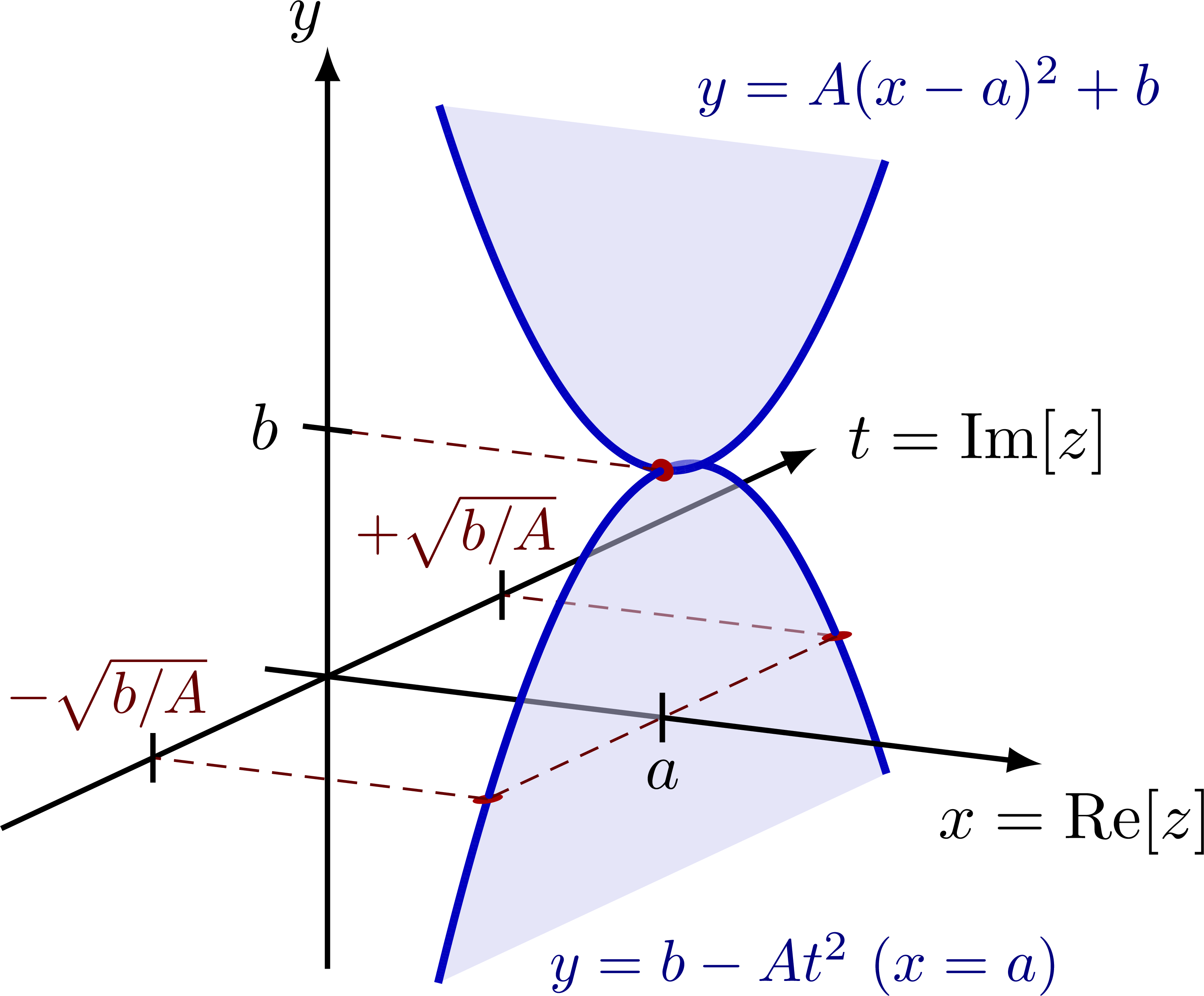
Take an upward (convex) parabola with a quadratic equation
\begin{equation}\label{real}
y = A(x-a)^2 + b,
\end{equation}
with real $A,b>0$.
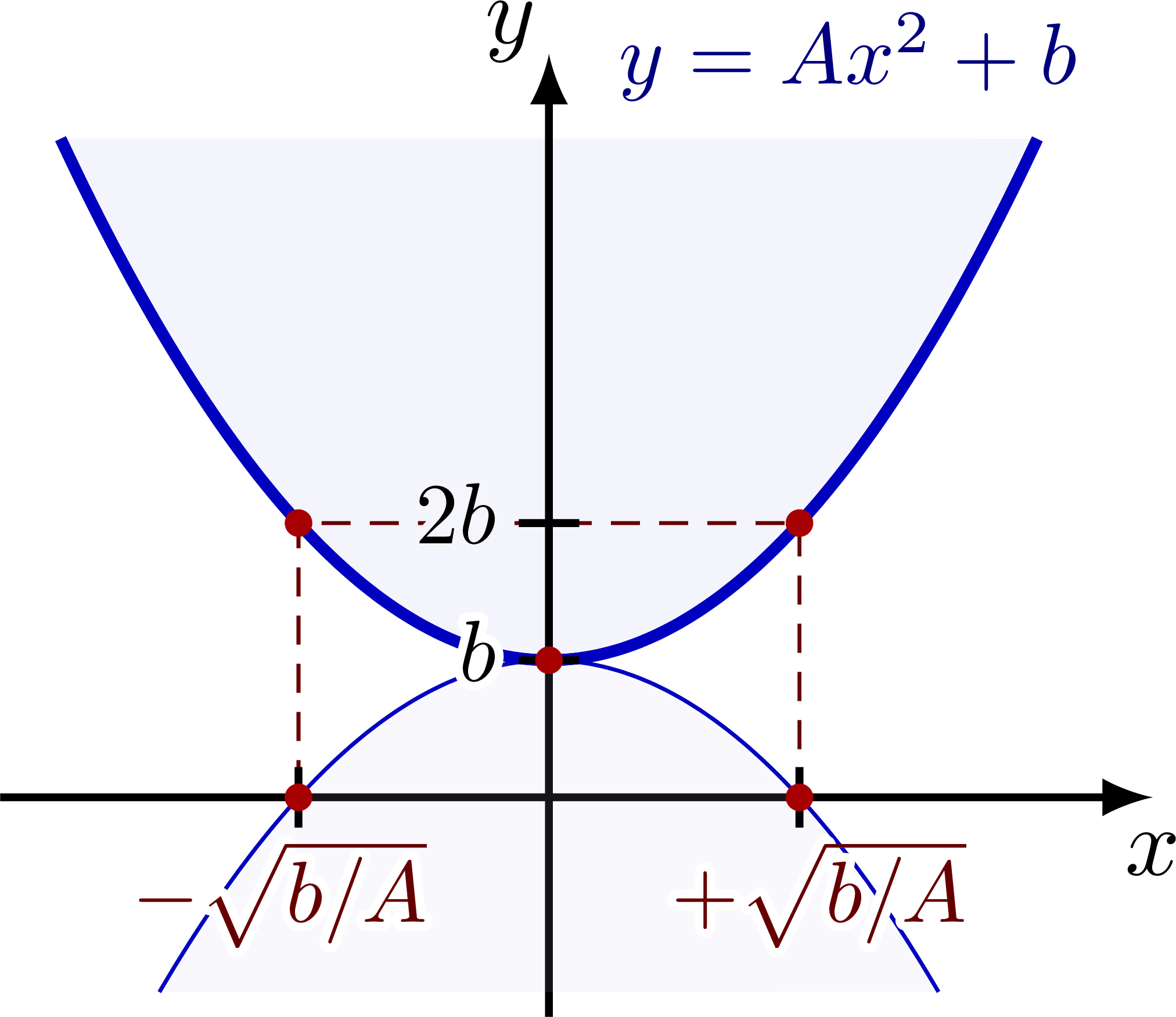
If $a=0$, there two imaginary roots
\begin{equation*}
x = \pm i\sqrt{\frac{b}{A}}.
\end{equation*}
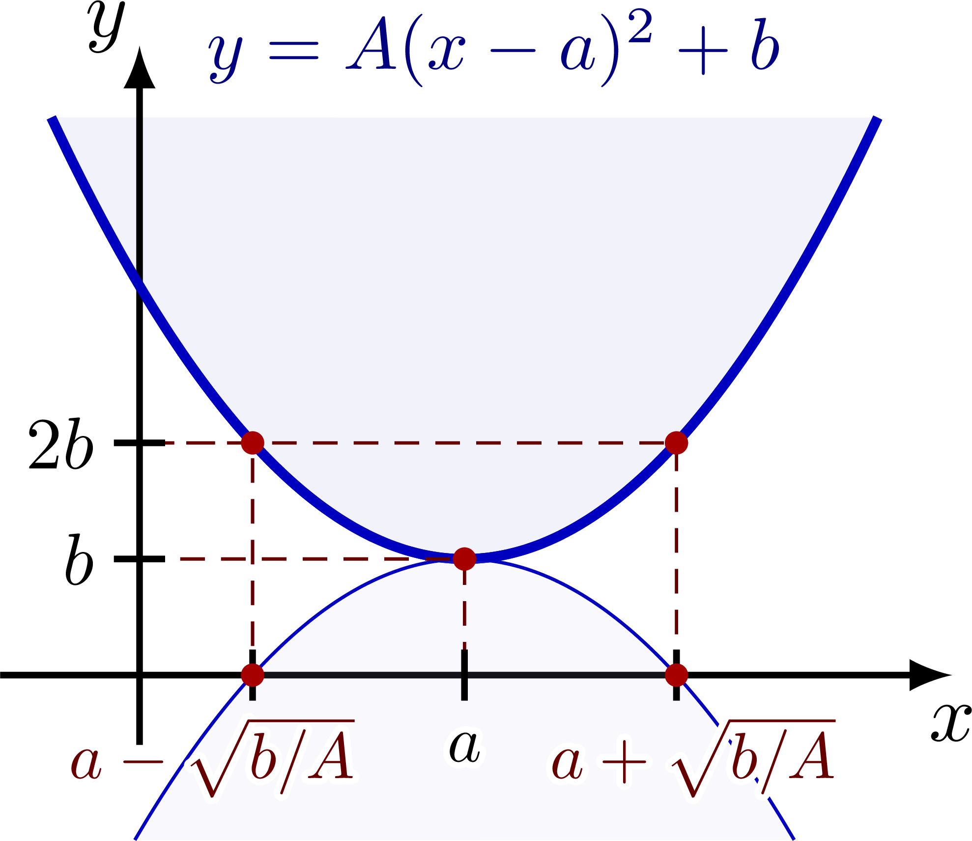
If $a\neq0$, there are two complex solutions
\begin{equation*}
x = a \pm i\sqrt{\frac{b}{A}}.
\end{equation*}
To extend the graph from the real $x$ axis to the complex plane,
substitute a complex number \mbox{$z = x + it$} for real $x$, $t$:
\begin{equation*}
y = \Re\!\big[ A(x+it-a)^2 + b \big].
\end{equation*}
Rewriting,
\begin{equation*}
y = \Re\!\big[ A(x-a)^2 -At^2 + b \big].
\end{equation*}
If $t=0$, we retrieve the ``real parabola'' \eqref{real}.
The ``complex parabola'' that has the same solution for $x=a$ is
\begin{equation*}
y = b -At^2.
\end{equation*}
\end{minipage}
};
\end{tikzpicture}
\end{document}Click to download: complex_roots.tex • complex_roots.pdf
Open in Overleaf: complex_roots.tex


")

