")


Some plots of basic electric circuits. Also see the related RC and RCL diagrams, or use the “circuits” tag.


Edit and compile if you like:
% Author: Izaak Neutelings (Februari, 2020)
\documentclass[border=3pt,tikz]{standalone}
\usepackage{amsmath} % for \dfrac
\usepackage{physics,siunitx}
\usepackage{tikz,pgfplots}
\usetikzlibrary{angles,quotes} % for pic (angle labels)
\usetikzlibrary{decorations.markings}
\tikzset{>=latex} % for LaTeX arrow head
\usepackage{xcolor}
\colorlet{Rcol}{green!60!black}
\colorlet{myblue}{blue!70!black}
\colorlet{myred}{red!70!black}
\colorlet{Ecol}{orange!90!black}
\tikzstyle{Rline}=[Rcol,thick]
\tikzstyle{gline}=[Rcol,thick]
\tikzstyle{bline}=[myblue,thick]
\tikzstyle{rline}=[myred,thick]
\def\xmax{4.5}
\def\ymax{3}
\def\tick#1#2{\draw[thick] (#1) ++ (#2:0.03*\ymax) --++ (#2-180:0.06*\ymax)}
\newcommand\EMF{\mathcal{E}} %\varepsilon}
\begin{document}
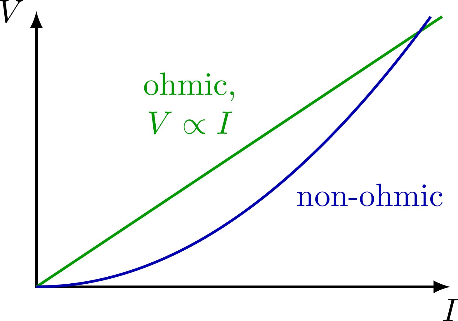
% OHMIC RESISTORS
\begin{tikzpicture}
\def\a{0.16}
\coordinate (O) at (0,0);
\coordinate (X) at (\xmax,0);
\coordinate (Y) at (0,\ymax);
% AXIS
\draw[<->,thick]
(X) node[below] {$I$} -- (O) -- (Y) node[left] {$V$};
% PLOT
\draw[Rline,samples=100,smooth,variable=\x,domain=0:0.98*\xmax]
plot(\x,\ymax/\xmax*\x);
\draw[bline,samples=100,smooth,variable=\x,domain=0:{sqrt(0.98*\ymax/\a)}]
plot(\x,\a*\x^2);
\node[Rcol,left,align=center] at (2.3,2.0) {ohmic,\\$V \propto I$};
\node[myblue,right] at (2.7,1.0) {non-ohmic};
\end{tikzpicture}
% RESISTIVITY
\begin{tikzpicture}
\def\a{\ymax/\xmax}
\def\Tz{0.5*\xmax}
\coordinate (O) at (0,0);
\coordinate (X) at (\xmax,0);
\coordinate (Y) at (0,\ymax);
\coordinate (P) at (\Tz,\a*\Tz);
\coordinate (Px) at (\Tz,0);
\coordinate (Py) at (0,\a*\Tz);
% AXIS
\draw[<->,thick]
(X) node[below] {$T$} -- (O) -- (Y) node[left] {$\rho$};
\tick{Px}{90} node[below] {$\SI{20}{\degree}$};
\tick{Py}{ 0} node[left] {$\rho_{20}$};
% PLOT
\draw[bline,samples=100,smooth,variable=\x,domain=0:0.98*\xmax]
plot(\x,\a*\x);
\draw[dashed] (Py) -- (P) -- (Px);
%\node[above right] at (1.4,1.8) {$E \sim \dfrac{1}{T}$};
\end{tikzpicture}
% RESISTIVITY
\begin{tikzpicture}
\def\a{2.4}
\coordinate (O) at (0,0);
\coordinate (X) at (\xmax,0);
\coordinate (Y) at (0,\ymax);
% AXIS
\draw[<->,thick]
(X) node[below] {$T$} -- (O) -- (Y) node[left] {$\rho$};
% PLOT
\draw[bline,samples=100,smooth,variable=\x,domain={1.1*\a/\ymax}:0.98*\xmax]
plot(\x,\a/\x);
%\node[above right] at (1.4,1.8) {$E \sim \dfrac{1}{T}$};
\end{tikzpicture}
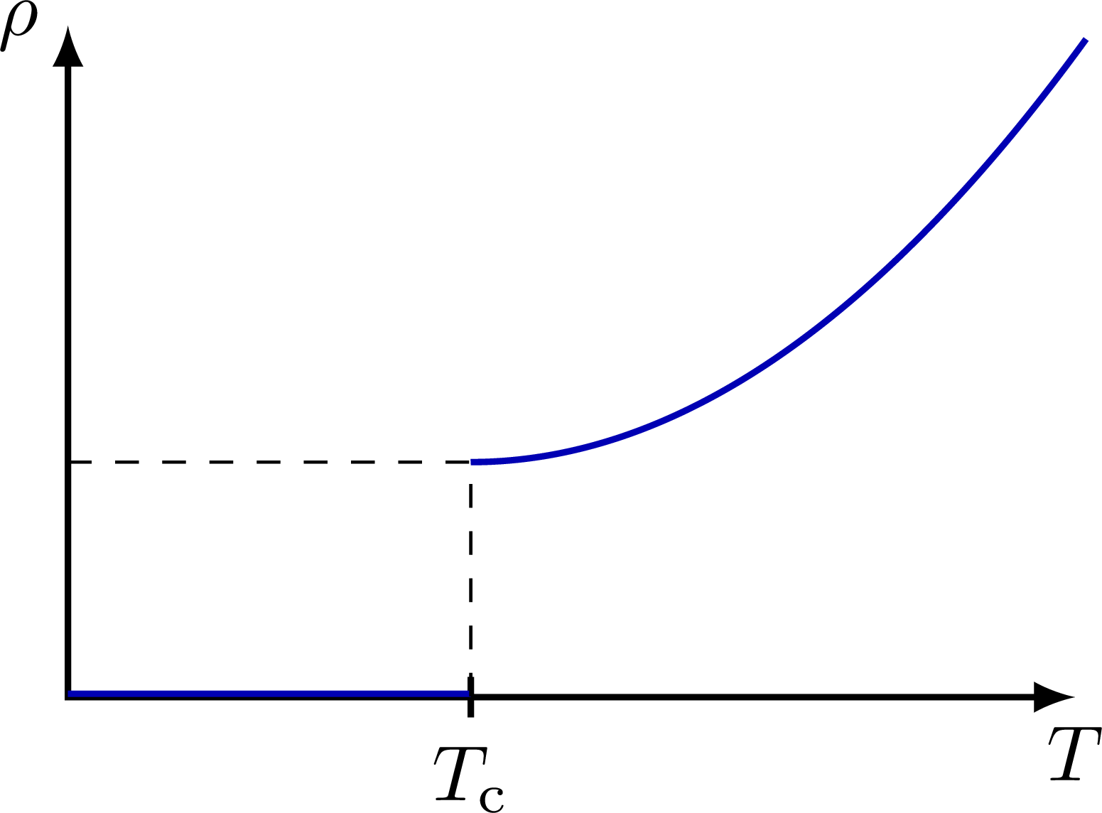
% RESISTIVITY
\begin{tikzpicture}
\def\a{0.25}
\def\Tc{1.8}
\def\rc{0.35*\ymax}
\coordinate (O) at (0,0);
\coordinate (X) at (\xmax,0);
\coordinate (Y) at (0,\ymax);
\coordinate (P) at (\Tc,\rc);
\coordinate (Px) at (\Tc,0);
\coordinate (Py) at (0,\rc);
% AXIS
\draw[<->,thick]
(X) node[below] {$T$} -- (O) -- (Y) node[left] {$\rho$};
%\tick{Py}{ 0} node[below=-1,left] {$\dfrac{kQ}{R^2}$};
\tick{Px}{90} node[below] {$T_\mathrm{c}$};
% PLOT
\draw[bline,samples=100,smooth,variable=\x,domain=\Tc:{sqrt((0.98*\ymax-\rc)/\a))+\Tc}]
plot(\x,{\rc+\a*(\x-\Tc)^2});
\draw[bline]
(0,0.005*\ymax) --++ (Px);
%\node[above right] at (2.8,1.6) {$E \sim \dfrac{1}{r^2}$};
\draw[dashed]
(Py) -- (P) -- (Px);
\end{tikzpicture}
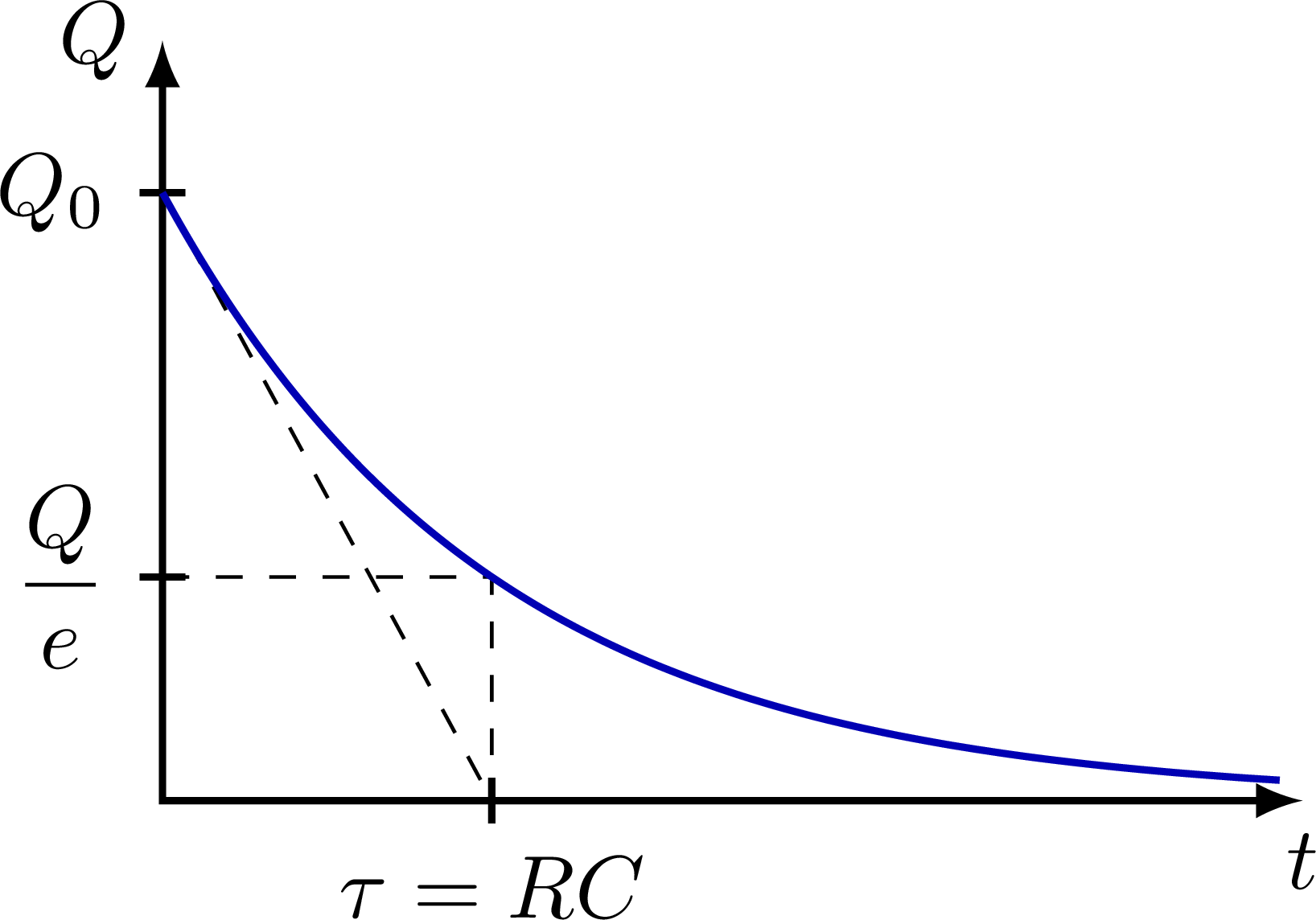
% RC circuit Q decharging
\begin{tikzpicture}
\def\a{2.4}
\def\t{1.3}
\coordinate (O) at (0,0);
\coordinate (X) at (\xmax,0);
\coordinate (Y) at (0,\ymax);
\coordinate (Q) at (0,\a);
\coordinate (T) at (\t,\a/2.718);
\coordinate (Tx) at (\t,0);
\coordinate (Ty) at (0,\a/2.718);
% AXIS
\draw[<->,thick]
(X) node[below] {$t$} -- (O) -- (Y) node[left] {$Q$};
\tick{Q}{0} node[left] {$Q_0$};
\tick{Tx}{90} node[below] {$\tau = RC$};
\tick{Ty}{0} node[left] {$\dfrac{Q}{e}$};
% PLOT
\draw[dashed] (Q) -- (Tx);
\draw[dashed] (Ty) -- (T) -- (Tx);
\draw[bline,samples=100,smooth,variable=\x,domain=0:0.98*\xmax]
plot(\x,{\a*exp(-\x/\t)});
\end{tikzpicture}
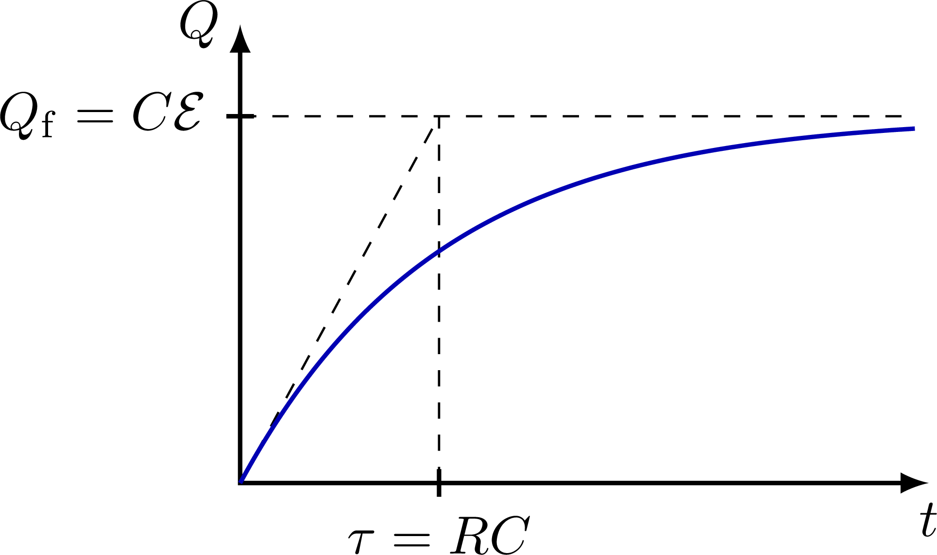
% RC circuit Q charging
\begin{tikzpicture}
\def\a{2.4}
\def\t{1.3}
\coordinate (O) at (0,0);
\coordinate (X) at (\xmax,0);
\coordinate (Y) at (0,\ymax);
\coordinate (Q) at (0,\a);
\coordinate (T) at (\t,\a);
\coordinate (Tx) at (\t,0);
% AXIS
\draw[<->,thick]
(X) node[below] {$t$} -- (O) -- (Y) node[left] {$Q$};
\tick{Q}{0} node[left] {$Q_\mathrm{f} = C\EMF$};
\tick{Tx}{90} node[below] {$\tau = RC$};
% PLOT
\draw[dashed] (Q) --++ (0.98*\xmax,0);
\draw[dashed] (Tx) -- (T);
\draw[dashed] (O) -- (T);
\draw[bline,samples=100,smooth,variable=\x,domain=0:0.98*\xmax]
plot(\x,{\a*(1-exp(-\x/\t)});
\end{tikzpicture}
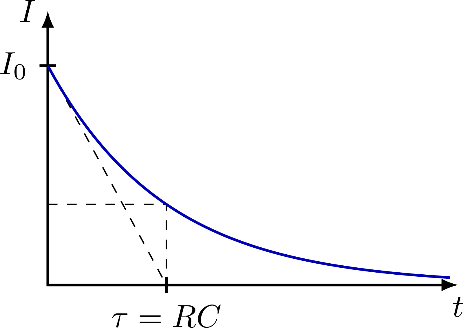
% RC circuit I charging
\begin{tikzpicture}
\def\a{2.4}
\def\t{1.3}
\coordinate (O) at (0,0);
\coordinate (X) at (\xmax,0);
\coordinate (Y) at (0,\ymax);
\coordinate (I) at (0,\a);
\coordinate (T) at (\t,\a/2.718);
\coordinate (Tx) at (\t,0);
\coordinate (Ty) at (0,\a/2.718);
% AXIS
\draw[<->,thick]
(X) node[below] {$t$} -- (O) -- (Y) node[left] {$I$};
\tick{I}{0} node[left] {$I_0$};
\tick{Tx}{90} node[below] {$\tau = RC$};
% PLOT
\draw[dashed] (I) -- (Tx);
\draw[dashed] (Ty) -- (T) -- (Tx);
\draw[bline,samples=100,smooth,variable=\x,domain=0:0.98*\xmax]
plot(\x,{\a*exp(-\x/\t)});
\end{tikzpicture}
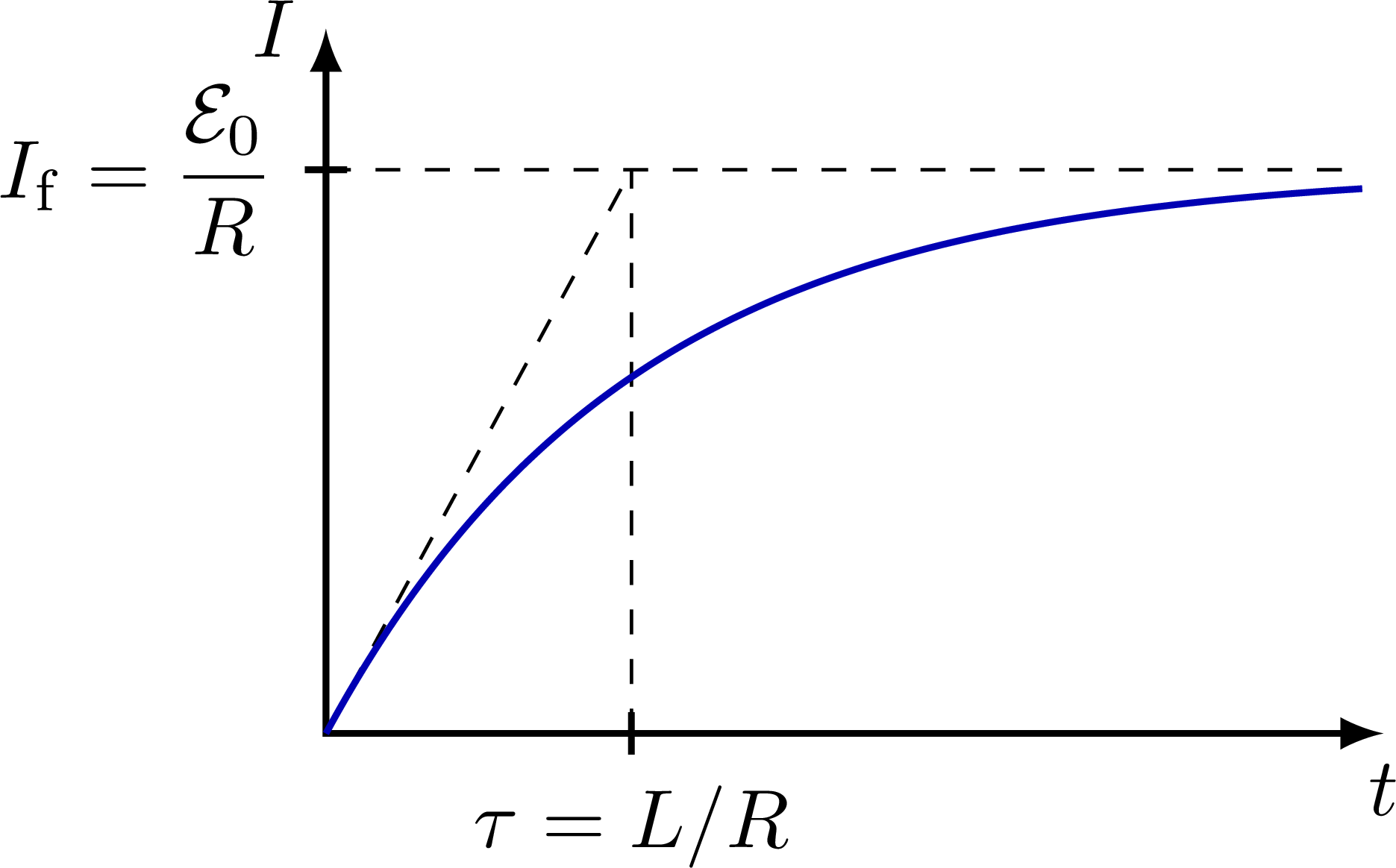
% RCL circuit I charging
\begin{tikzpicture}
\def\a{2.4}
\def\t{1.3}
\coordinate (O) at (0,0);
\coordinate (X) at (\xmax,0);
\coordinate (Y) at (0,\ymax);
\coordinate (I) at (0,\a);
\coordinate (T) at (\t,\a);
\coordinate (Tx) at (\t,0);
% AXIS
\draw[<->,thick]
(X) node[below] {$t$} -- (O) -- (Y) node[left] {$I$};
\tick{Q}{0} node[left] {$I_\mathrm{f} = \dfrac{\EMF_0}{R}$};
\tick{Tx}{90} node[below] {$\tau = L/R$};
% PLOT
\draw[dashed] (I) --++ (0.98*\xmax,0);
\draw[dashed] (Tx) -- (T);
\draw[dashed] (O) -- (T);
\draw[bline,samples=100,smooth,variable=\x,domain=0:0.98*\xmax]
plot(\x,{\a*(1-exp(-\x/\t)});
\end{tikzpicture}
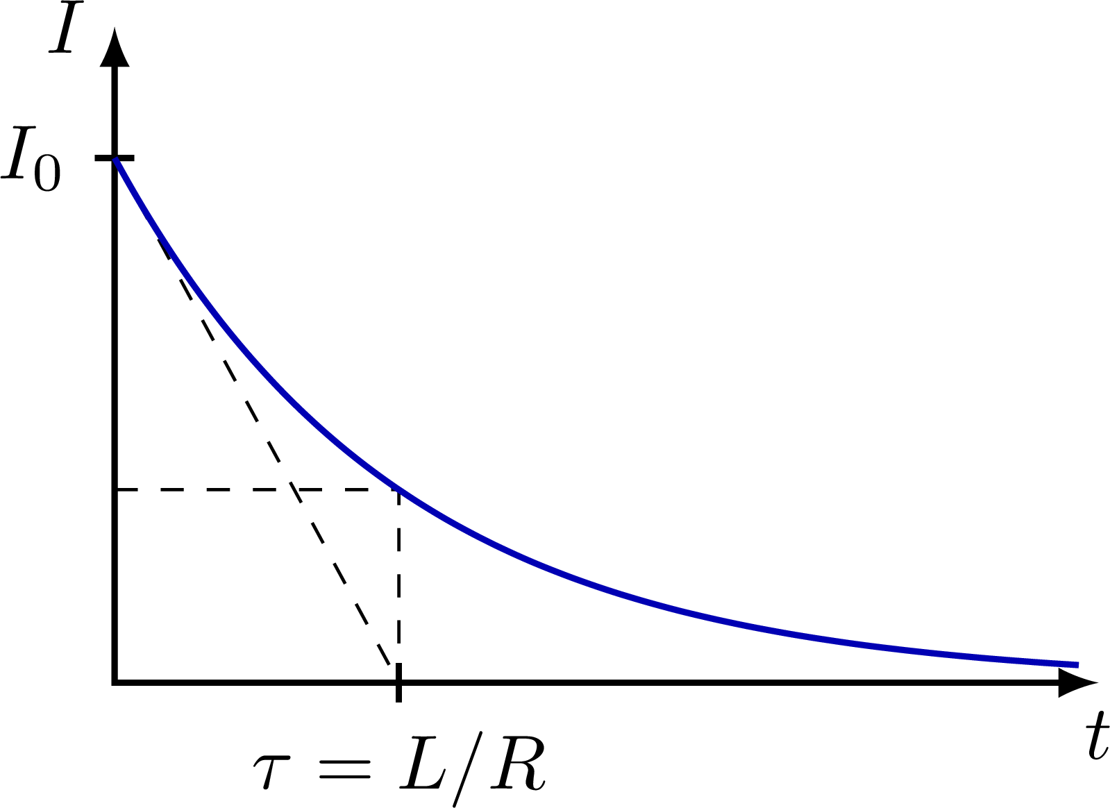
% RC circuit I discharging
\begin{tikzpicture}
\def\a{2.4}
\def\t{1.3}
\coordinate (O) at (0,0);
\coordinate (X) at (\xmax,0);
\coordinate (Y) at (0,\ymax);
\coordinate (I) at (0,\a);
\coordinate (T) at (\t,\a/2.718);
\coordinate (Tx) at (\t,0);
\coordinate (Ty) at (0,\a/2.718);
% AXIS
\draw[<->,thick]
(X) node[below] {$t$} -- (O) -- (Y) node[left] {$I$};
\tick{I}{0} node[left] {$I_0$};
\tick{Tx}{90} node[below] {$\tau = L/R$};
% PLOT
\draw[dashed] (I) -- (Tx);
\draw[dashed] (Ty) -- (T) -- (Tx);
\draw[bline,samples=100,smooth,variable=\x,domain=0:0.98*\xmax]
plot(\x,{\a*exp(-\x/\t)});
\end{tikzpicture}
% RCL circuit V, Q alternating
\begin{tikzpicture}
%\def\xmax{9}
\def\ymax{1.6}
\def\a{1.2}
\def\t{360/(0.94*\xmax)}
\coordinate (O) at (0,0);
\coordinate (X) at (\xmax,0);
\coordinate (Y) at (0,\ymax);
% AXIS
\draw[->,thick]
(0,-\ymax) -- (Y) node[left] {$V$, $Q$};
\draw[->,thick]
(O) -- (X) node[below] {$t$};
% PLOT
\draw[bline,samples=100,smooth,variable=\x,domain=0:0.94*\xmax]
plot(\x,{\a*cos(\t*\x)});
\end{tikzpicture}
% RCL circuit I alternating
\begin{tikzpicture}
%\def\xmax{9}
\def\ymax{1.6}
\def\a{1.2}
\def\t{360/(0.94*\xmax)}
\coordinate (O) at (0,0);
\coordinate (X) at (\xmax,0);
\coordinate (Y) at (0,\ymax);
% AXIS
\draw[->,thick]
(0,-\ymax) -- (Y) node[left] {$I$};
\draw[->,thick]
(O) -- (X) node[below] {$t$};
% PLOT
\draw[bline,samples=100,smooth,variable=\x,domain=0:0.94*\xmax]
plot(\x,{-\a*sin(\t*\x)});
\end{tikzpicture}
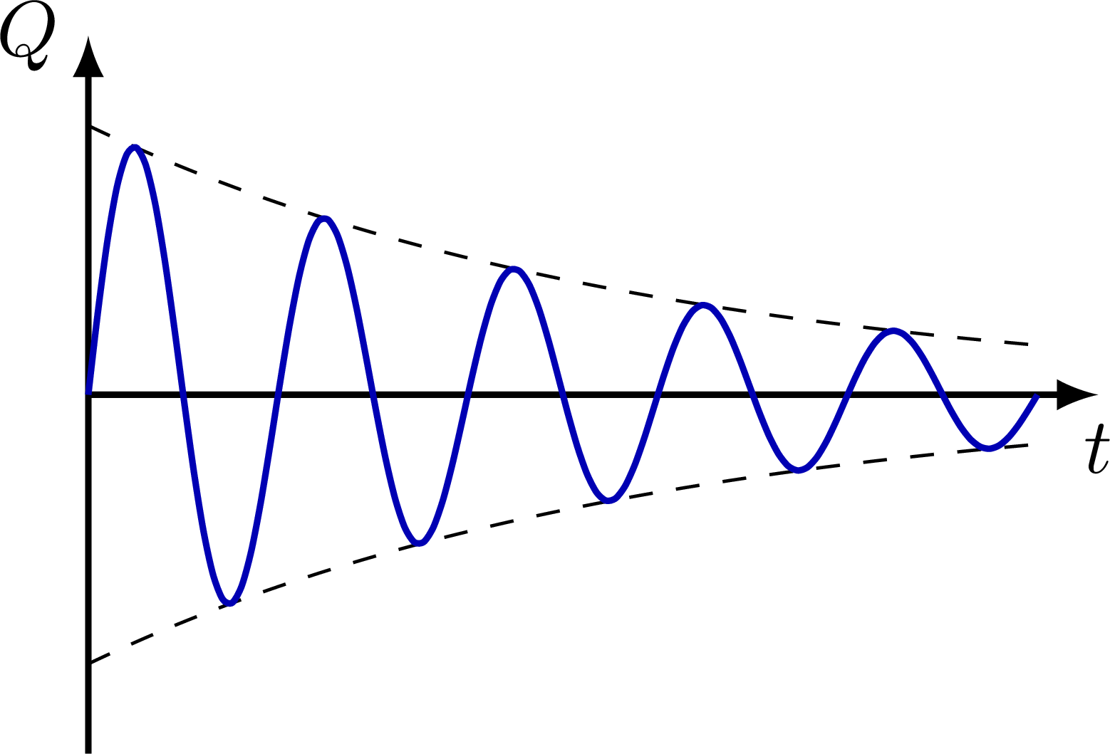
% RCL circuit Q alternating, exponential
\begin{tikzpicture}
%\def\xmax{9}
\def\ymax{1.6}
\def\a{1.2}
\def\t{1800/(0.94*\xmax)}
\def\T{0.4}
\coordinate (O) at (0,0);
\coordinate (X) at (\xmax,0);
\coordinate (Y) at (0,\ymax);
% AXIS
\draw[->,thick]
(0,-\ymax) -- (Y) node[left] {$Q$};
\draw[->,thick]
(O) -- (X) node[below] {$t$};
% PLOT
\draw[dashed,samples=100,smooth,variable=\x,domain=0:0.94*\xmax]
plot(\x,{\a*exp(-\T*\x)}) plot(\x,{-\a*exp(-\T*\x)});
\draw[bline,samples=100,smooth,variable=\x,domain=0:0.94*\xmax]
plot(\x,{\a*exp(-\T*\x)*sin(\t*\x)});
\end{tikzpicture}
\end{document}
Click to download: electric_circuit_plots.tex • electric_circuit_plots.pdf
Open in Overleaf: electric_circuit_plots.tex


