Gaussian distributions & statistical tests

Normal/gaussian/bell curve distributions and more to illustrate probability density functions (pdfs), sigma bands (68-95-99 rule), test statistics, critical regions (accept/reject), type-I and type-II errors (alpha, beta), null hypothesis tests, p-value, low sensitivity, bias & systematic error, S+B vs. B-only hypotheses, upper limits and the CLs method.

Inspired by Glen Cowen’s CERN lectures and this Higgs physics course by Mauro Donega at the UZH & ETHZ. Presented in this talk on the statistical method in particle physics.

Also see critical regions and these sets of critical regions.

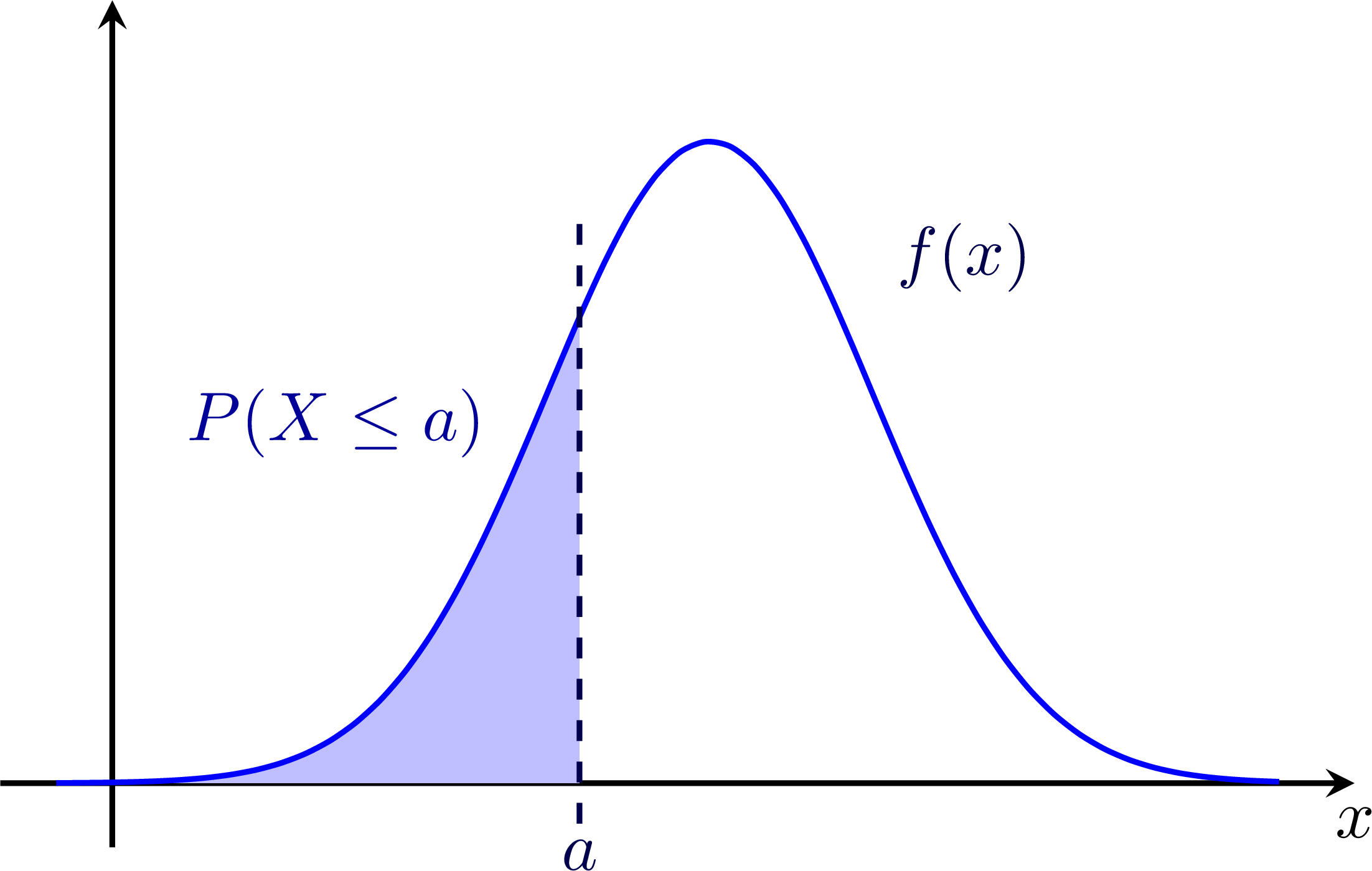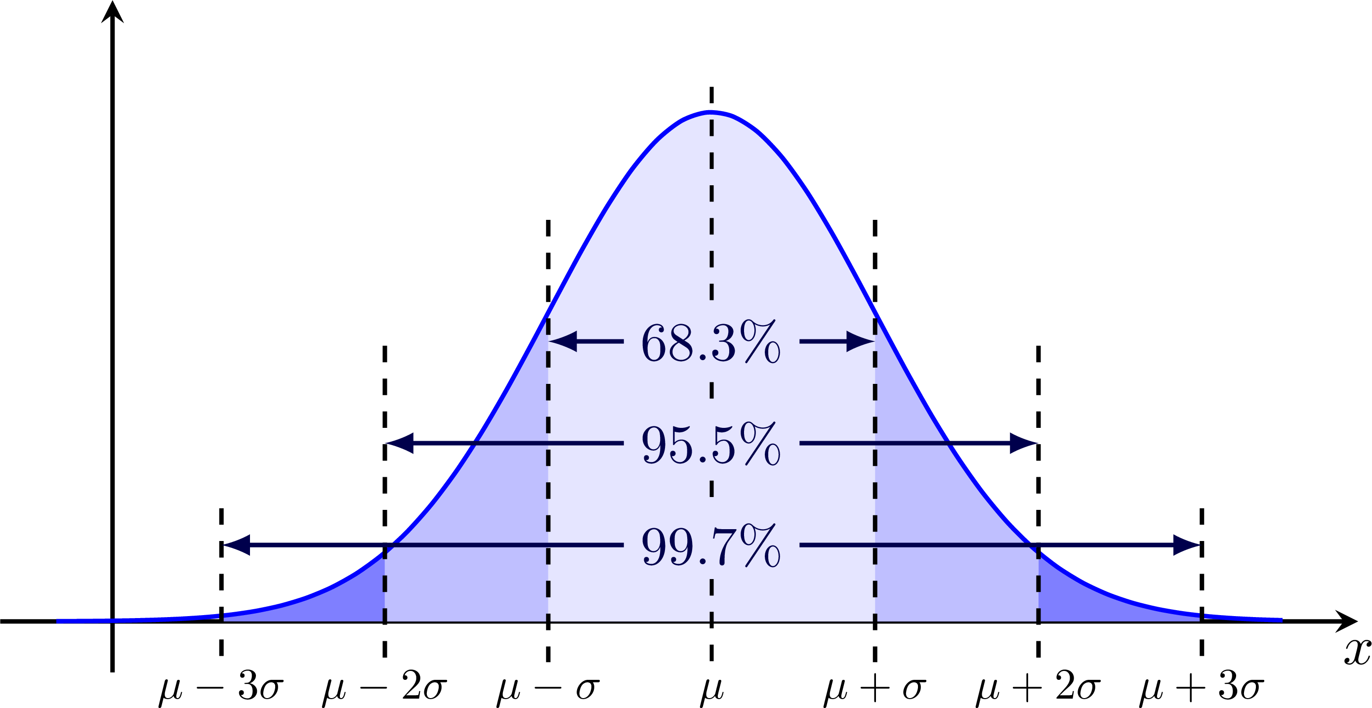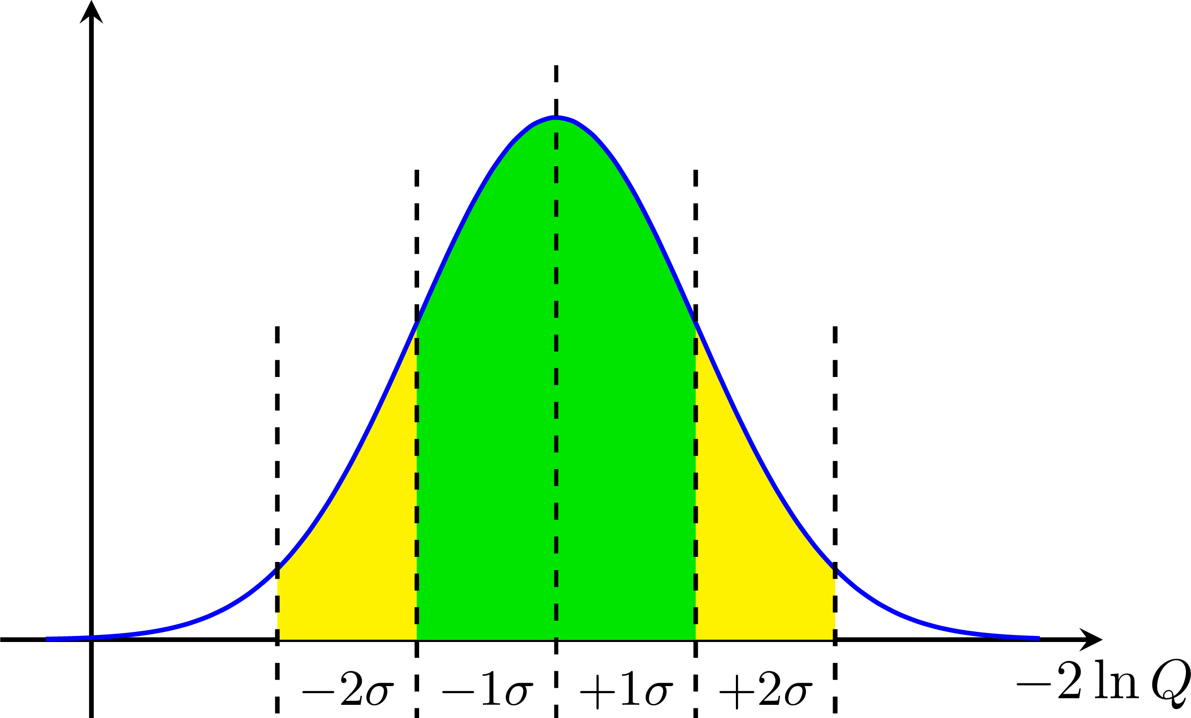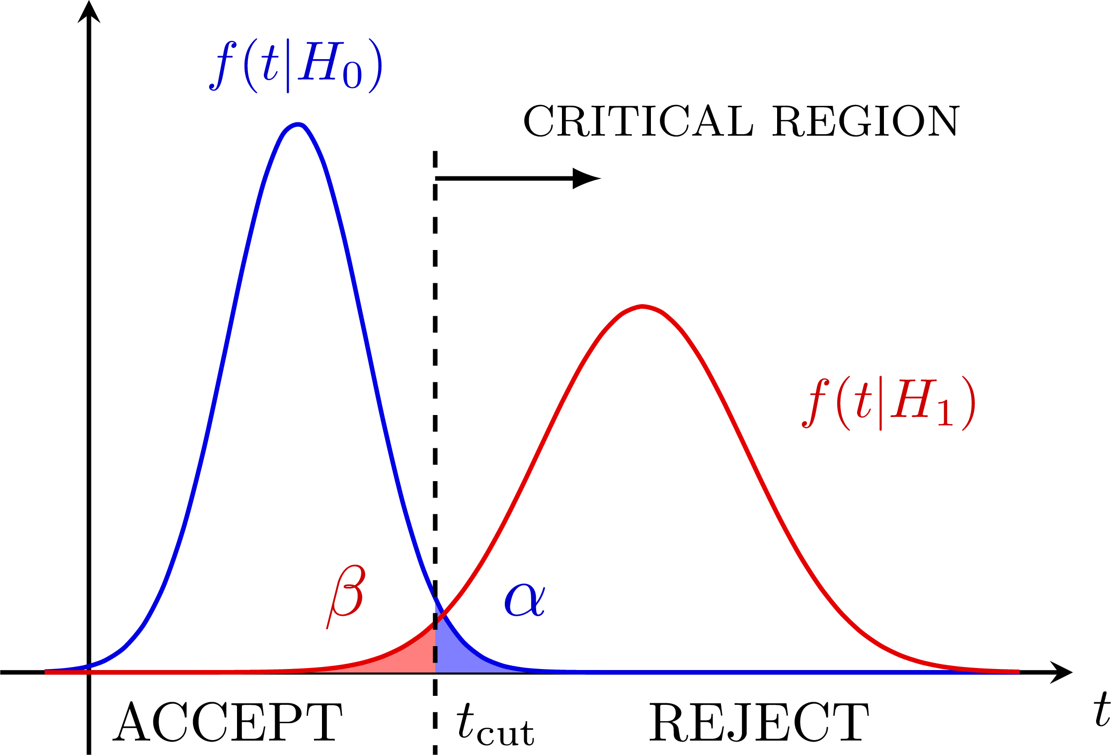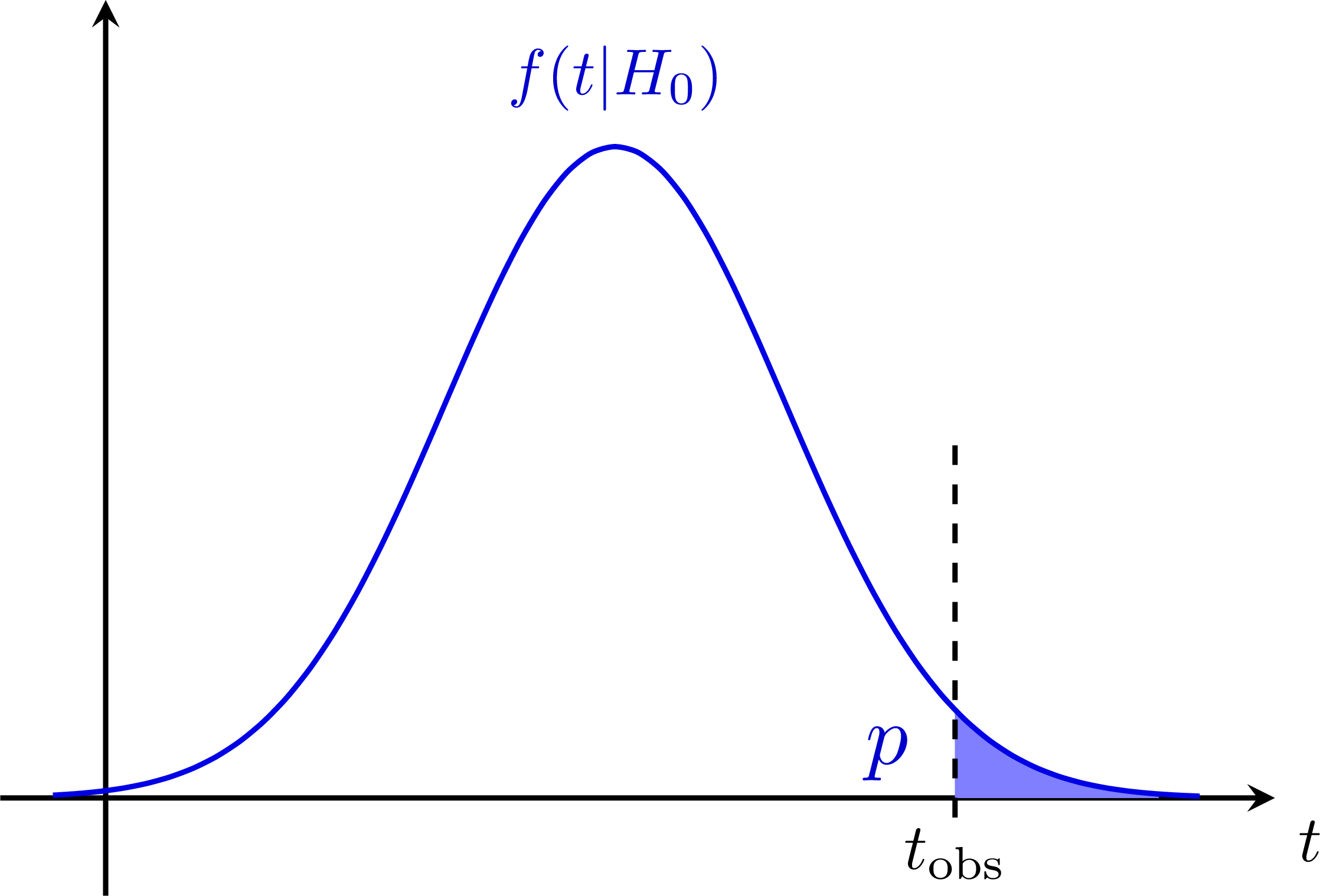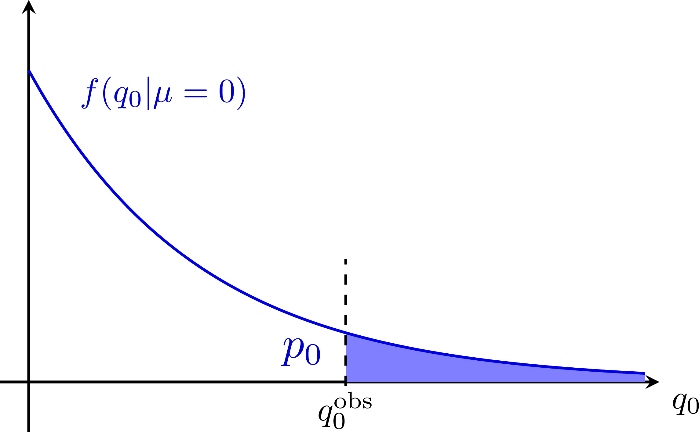
Probability from gaussian probability density functions (pdfs):The 68-95-99 rule:Sigma (standard deviation) bands for 'Brazilian flag' plots:Hypothesis testing with a test statistics t to define a critical region (accept/reject) with type-I (alpha) and type-II errors (beta):P-value (for a null-hypothesis):P-value for a B-only model (signal strength μ = 0): 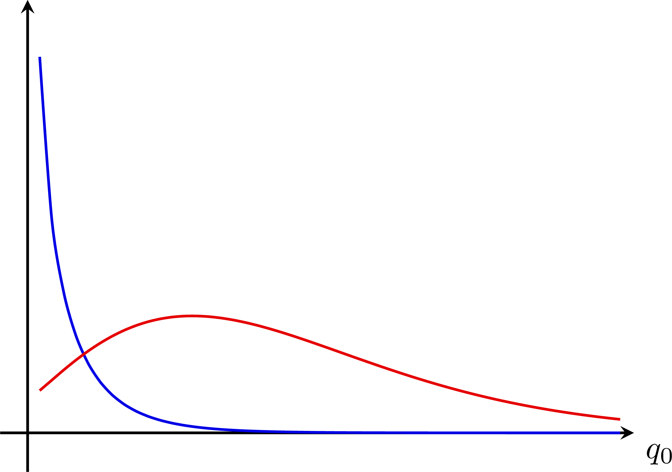P-value for an S+B and B-only hypothesis: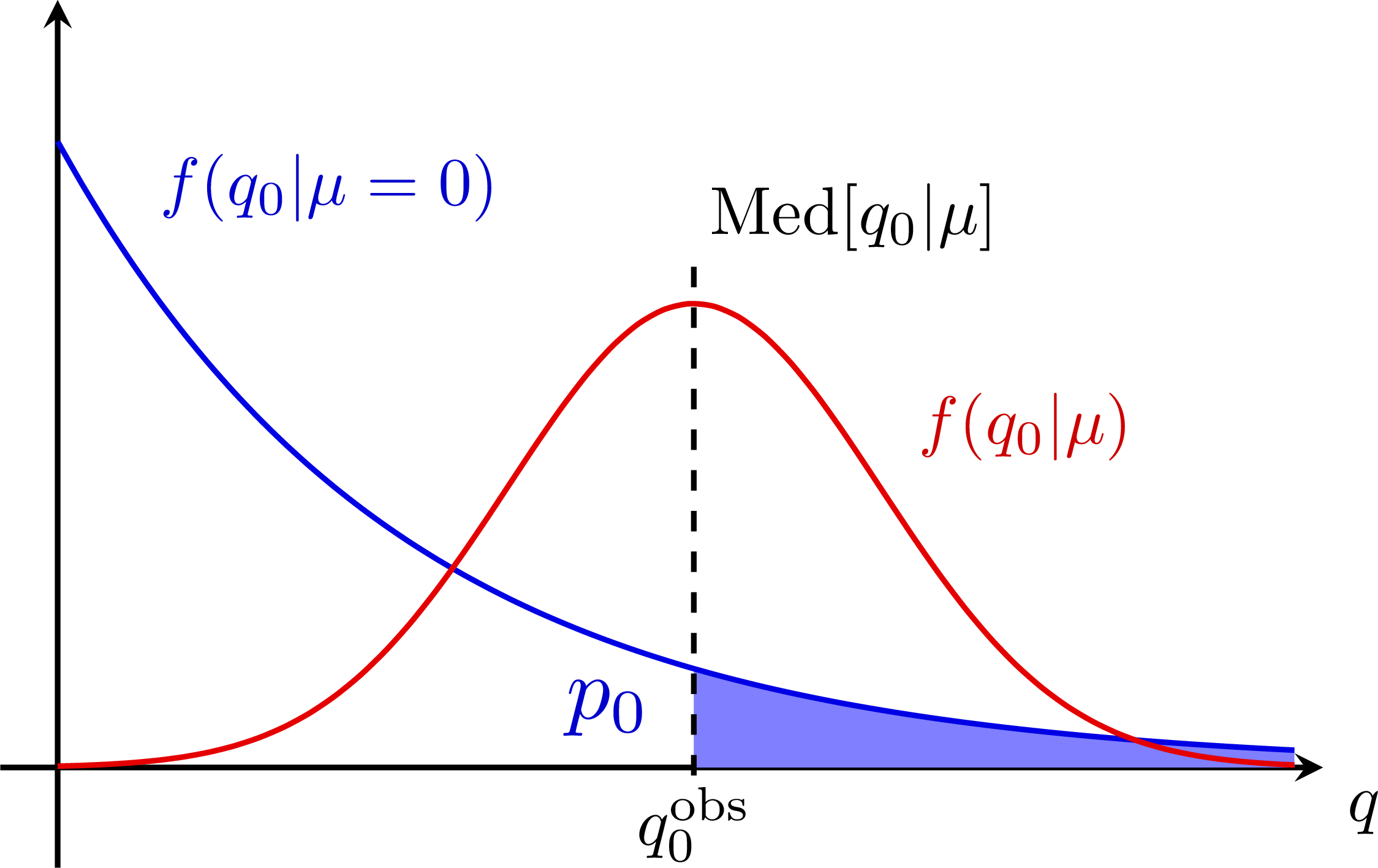Bias & systematic error from nuisance parameters: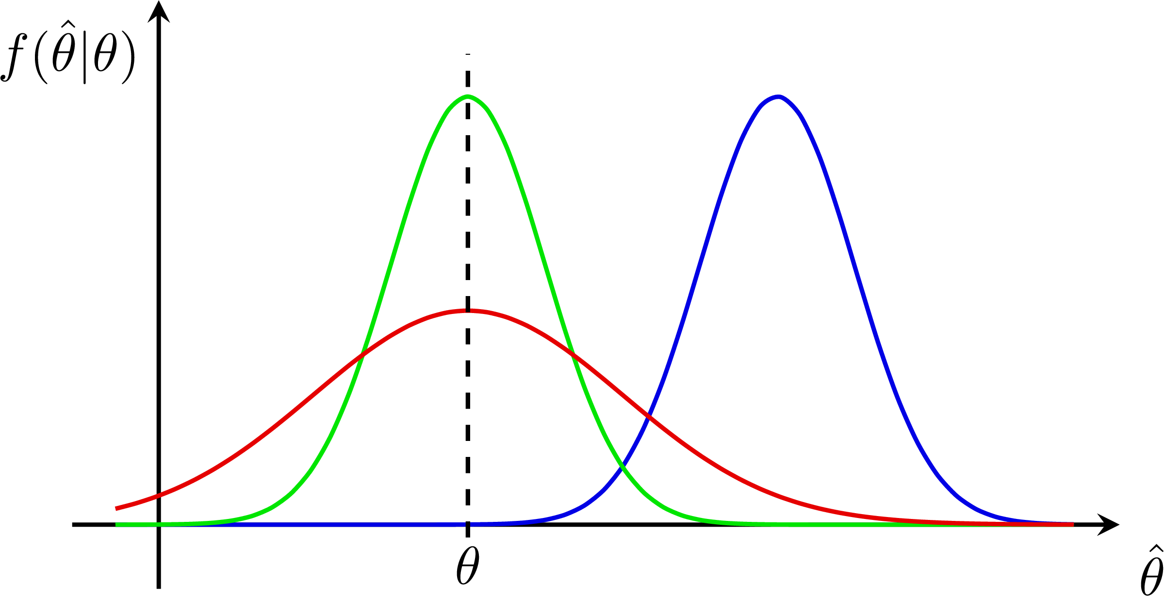Z-scores for a normal distribution: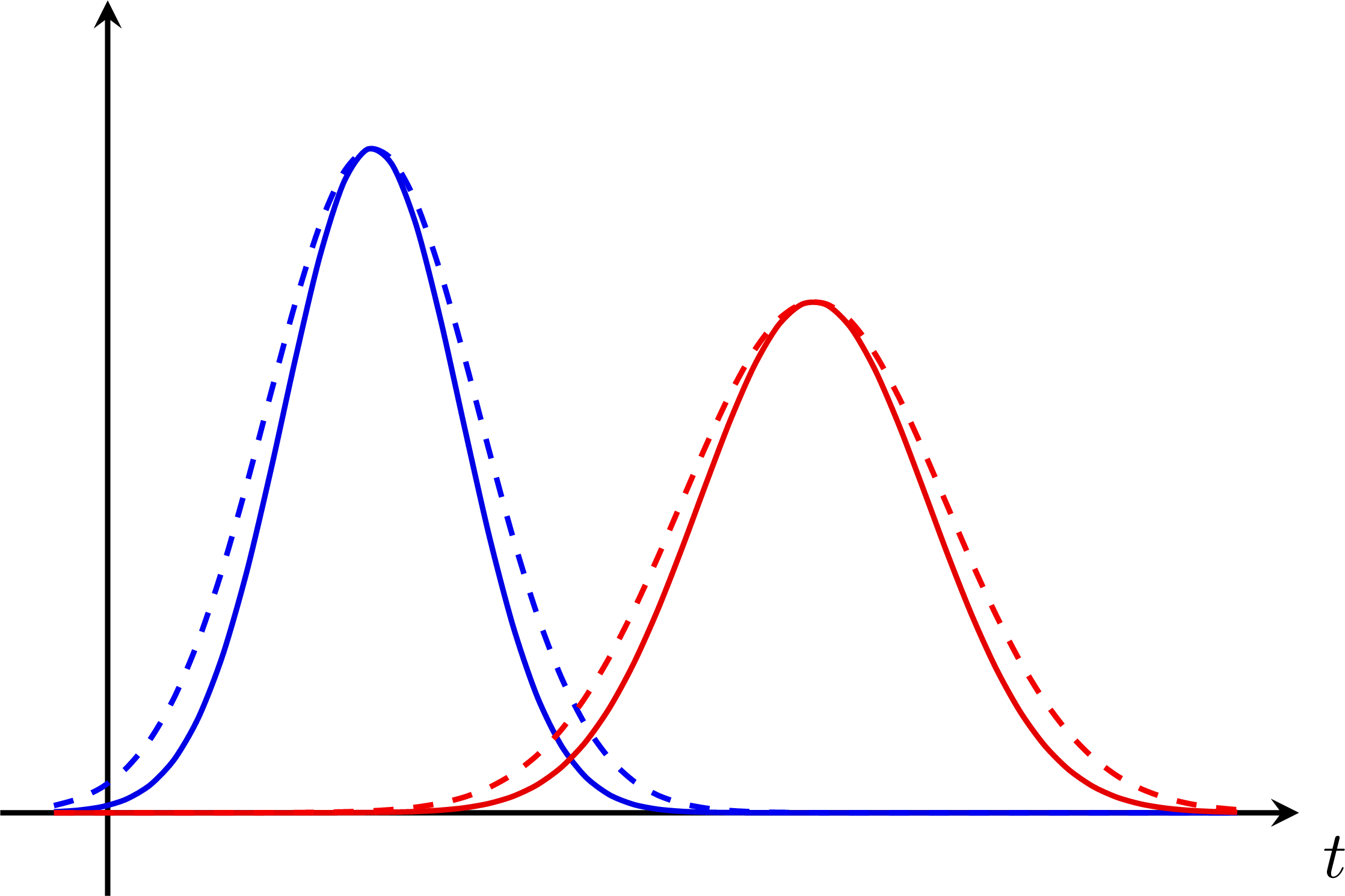Hypothesis testing with null-hypothesis H0: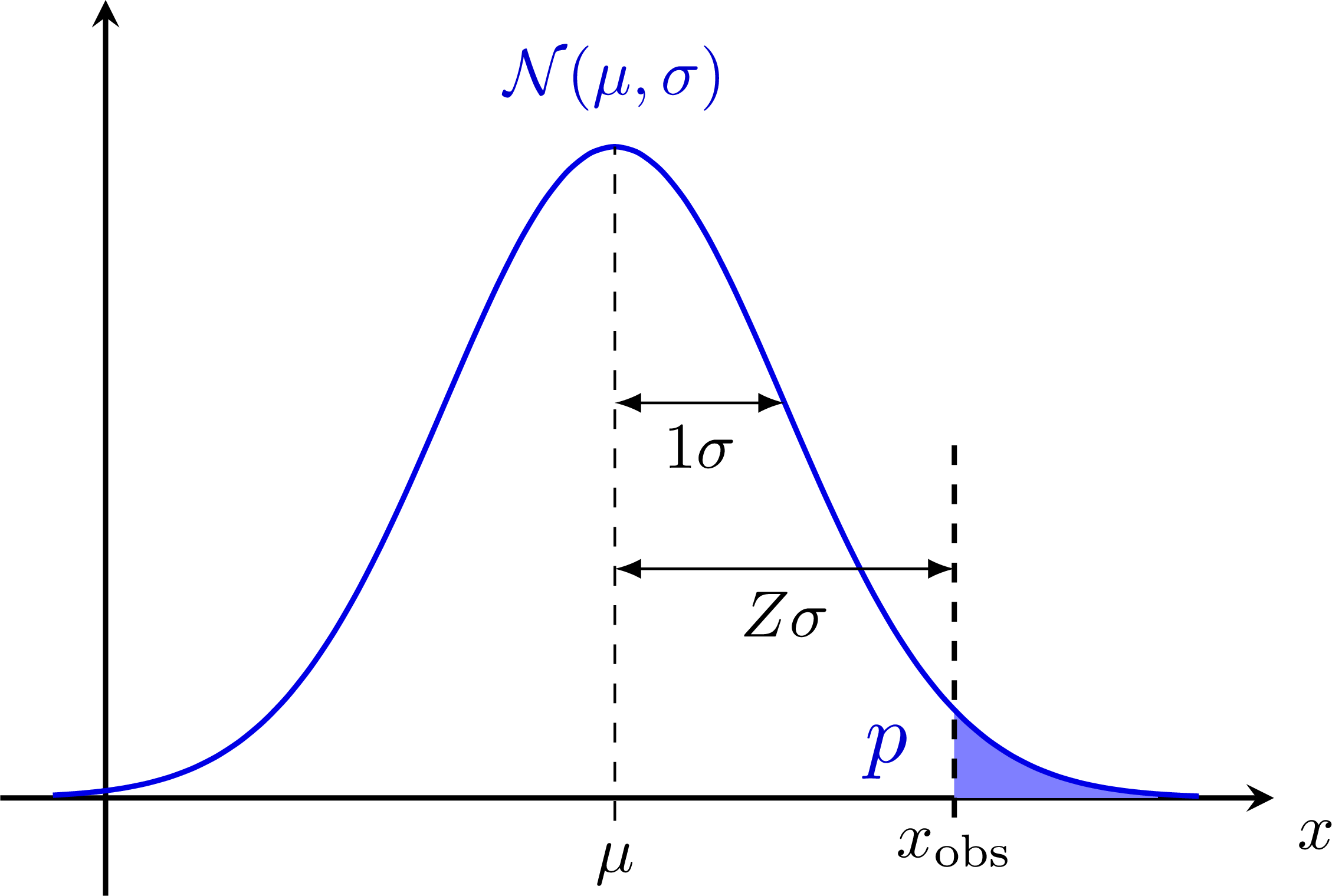Hypothesis testing with two gaussians: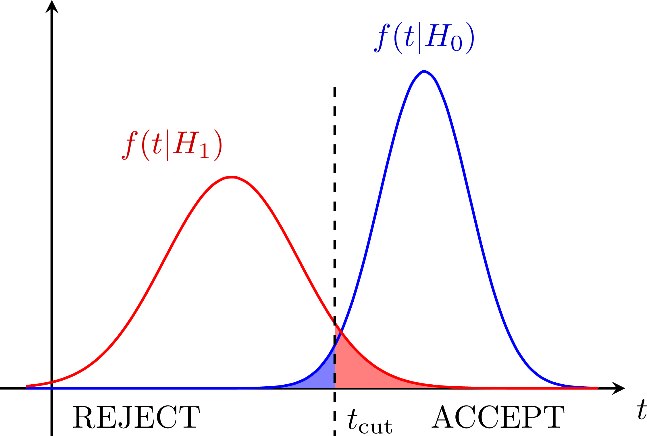Test power: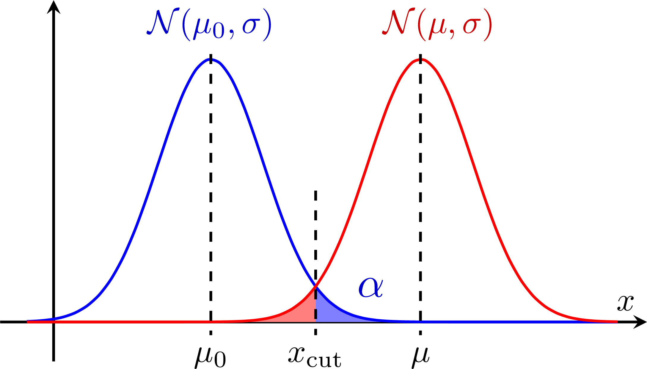Low power/sensitivity: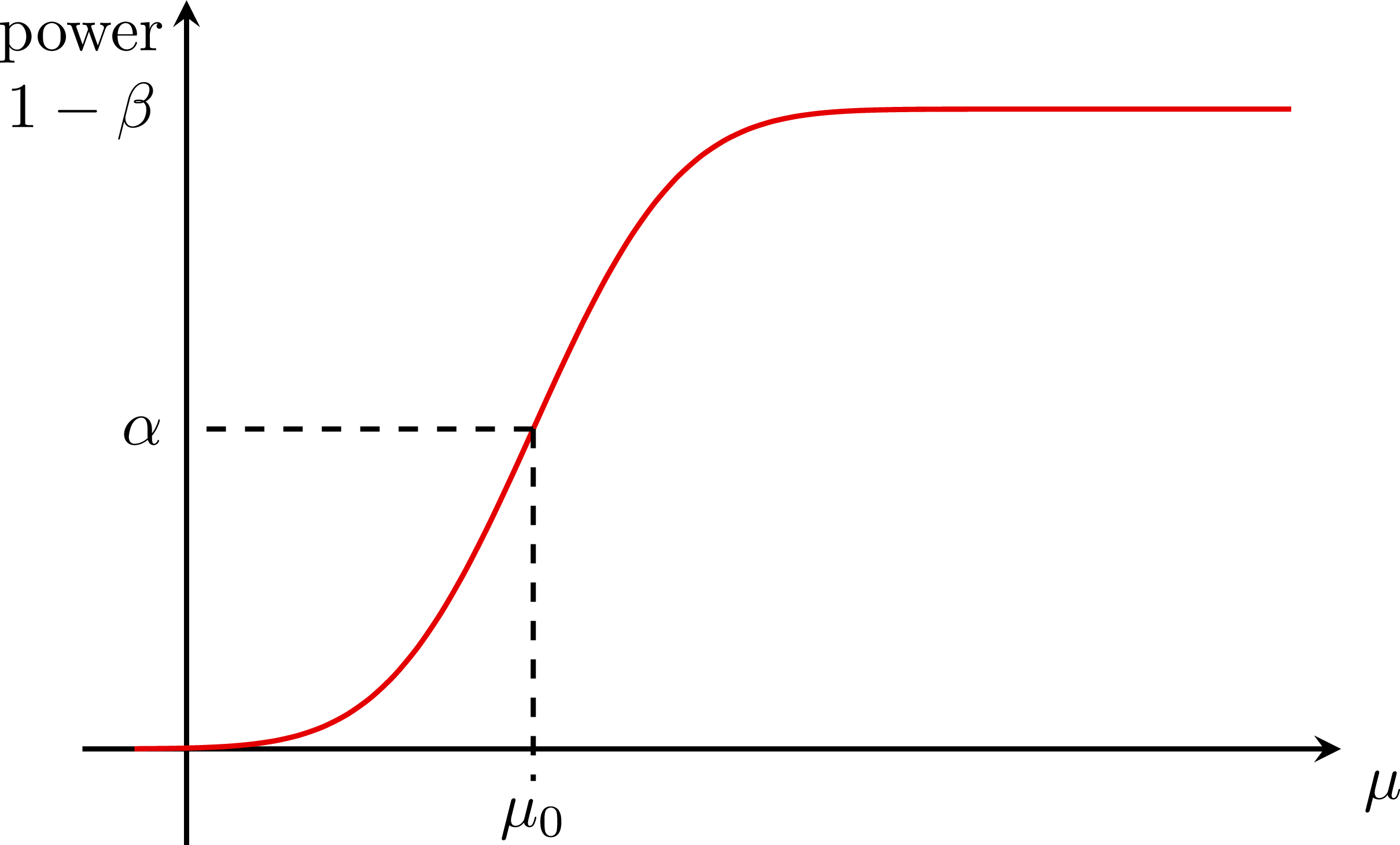Better power: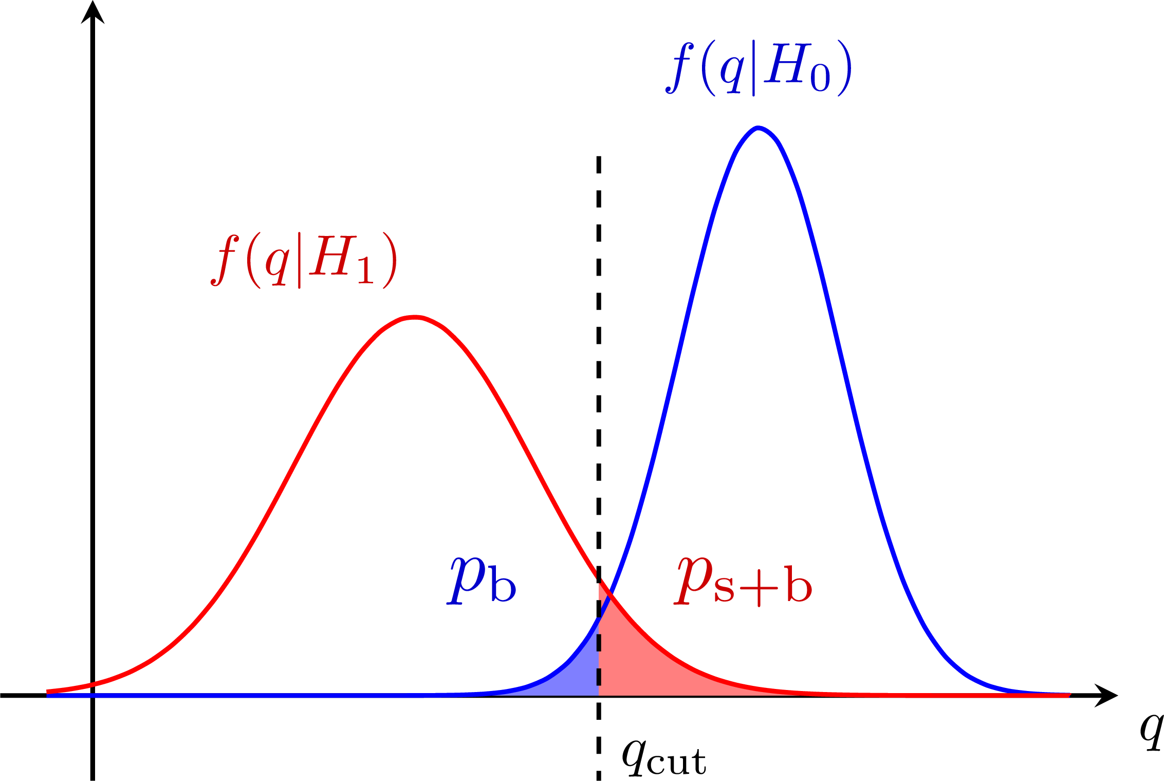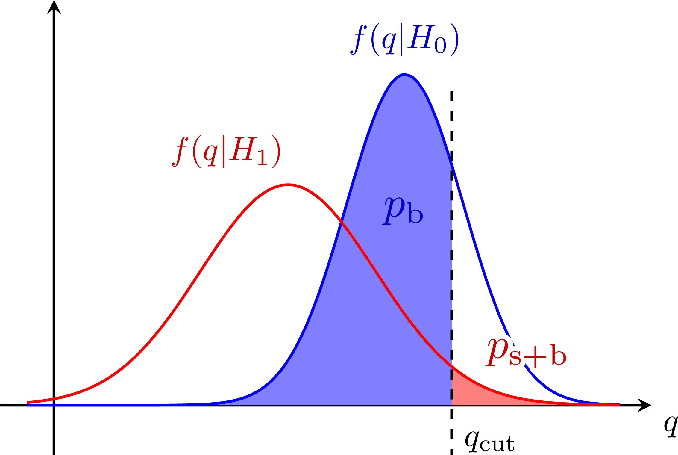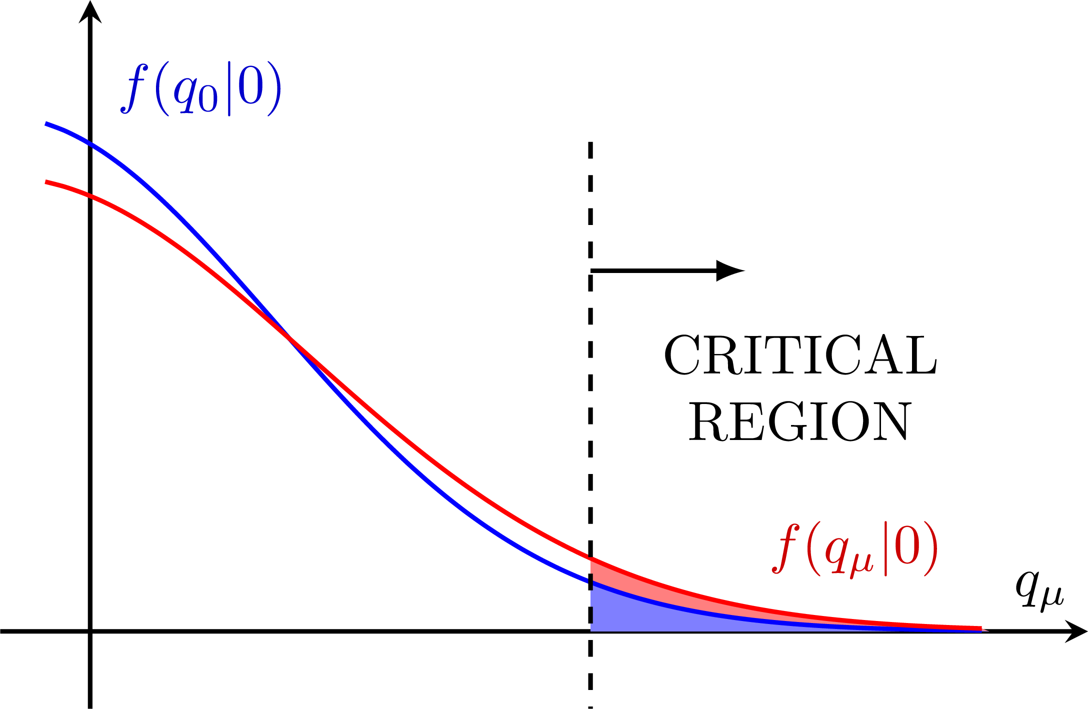S+B and B-only p-values for the CLs method:

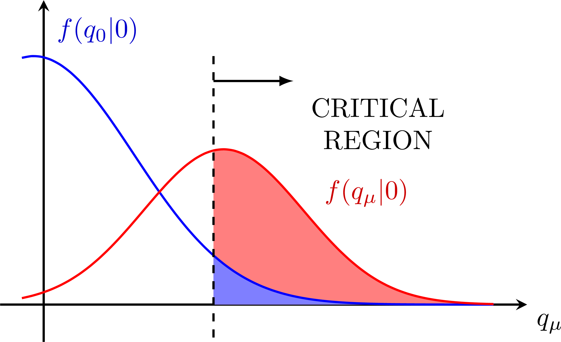
Edit and compile if you like:

1
2
3
4
5
6
7
8
9
10
11
12
13
14
15
16
17
18
19
20
21
22
23
24
25
26
27
28
29
30
31
32
33
34
35
36
37
38
39
40
41
% Author: Izaak Neutelings (August, 2017)
\documentclass[border=3pt,tikz]{standalone} %[dvipsnames]
\usepackage{amsmath} % for \dfrac
\usepackage{tikz}
\tikzset{>=latex} % for LaTeX arrow head
\usepackage{pgfplots} % for the axis environment
\usepackage{xcolor}
\usepackage[outline]{contour} % halo around text
\contourlength{1.2pt}
\usetikzlibrary{positioning,calc}
\usetikzlibrary{backgrounds}% required for 'inner frame sep'
%\usepackage{adjustbox} % add whitespace (trim)
% define gaussian pdf and cdf
\pgfmathdeclarefunction{gauss}{3}{%
  \pgfmathparse{1/(#3*sqrt(2*pi))*exp(-((#1-#2)^2)/(2*#3^2))}%
}
\pgfmathdeclarefunction{cdf}{3}{%
  \pgfmathparse{1/(1+exp(-0.07056*((#1-#2)/#3)^3 - 1.5976*(#1-#2)/#3))}%
}
\pgfmathdeclarefunction{fq}{3}{%
  \pgfmathparse{1/(sqrt(2*pi*#1))*exp(-(sqrt(#1)-#2/#3)^2/2)}%
}
\pgfmathdeclarefunction{fq0}{1}{%
  \pgfmathparse{1/(sqrt(2*pi*#1))*exp(-#1/2))}%
}
\colorlet{mydarkblue}{blue!30!black}
% to fill an area under function
\usepgfplotslibrary{fillbetween}
\usetikzlibrary{patterns}
\pgfplotsset{compat=1.12} % TikZ coordinates <-> axes coordinates
% https://tex.stackexchange.com/questions/240642/add-vertical-line-of-equation-x-2-and-shade-a-region-in-graph-by-pgfplots
% plot aspect ratio
%\def\axisdefaultwidth{8cm}
%\def\axisdefaultheight{6cm}
 
 
הההההההההההההההההההההההההההההההההההההההההההההההההההההההההההההההההההההההההההההההההההההההההההההההההההההההההההההההההההההההההההההההההההההההההההההההההההההההההההההההההההההההההההההההההההההההההההההההההההההההההההההההההההההההההההההההההההההההההההההההההההההההההההההההה
XXXXXXXXXXXXXXXXXXXXXXXXXXXXXXXXXXXXXXXXXXXXXXXXXXXXXXXXXXXXXXXXXXXXXXXXXXXXXXXXXXXXXXXXXXXXXXXXXXXXXXXXXXXXXXXXXXXXXXXXXXXXXXXXXXXXXXXXXXXXXXXXXXXXXXXXXXXXXXXXXXXXXXXXXXXXXXXXXXXXXXXXXXXXXXXXXXXXXXXXXXXXXXXXXXXXXXXXXXXXXXXXXXXXXXXXXXXXXXXXXXXXXXXXXXXXXXXX

Run LaTeX here
Click to download: gaussians.tex • gaussians.pdf
Open in Overleaf: gaussians.tex