")


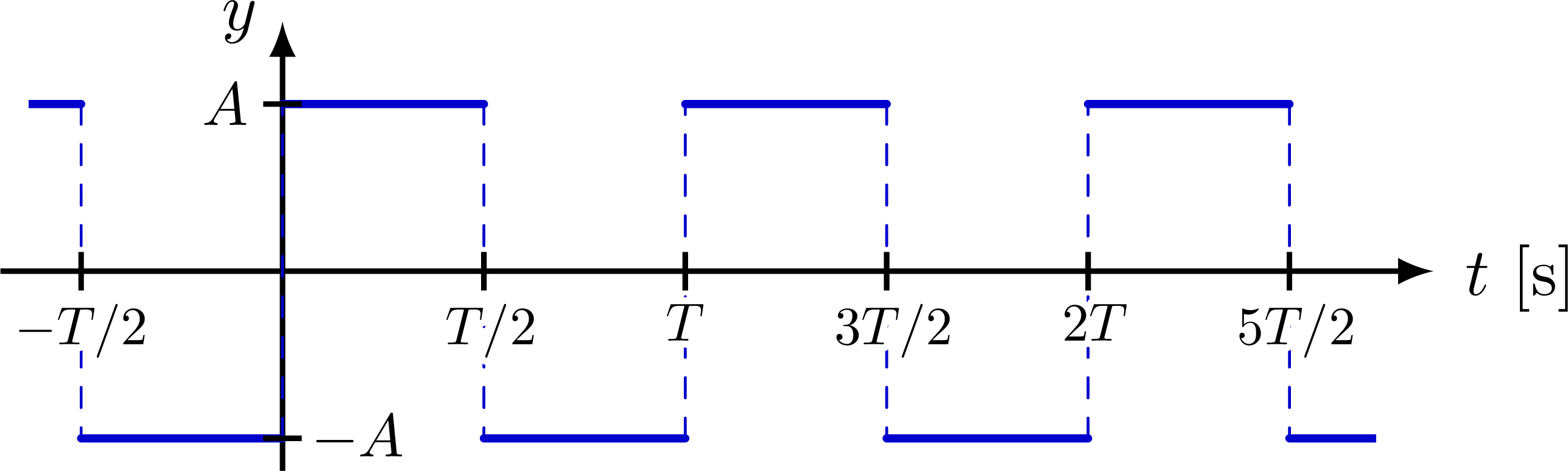
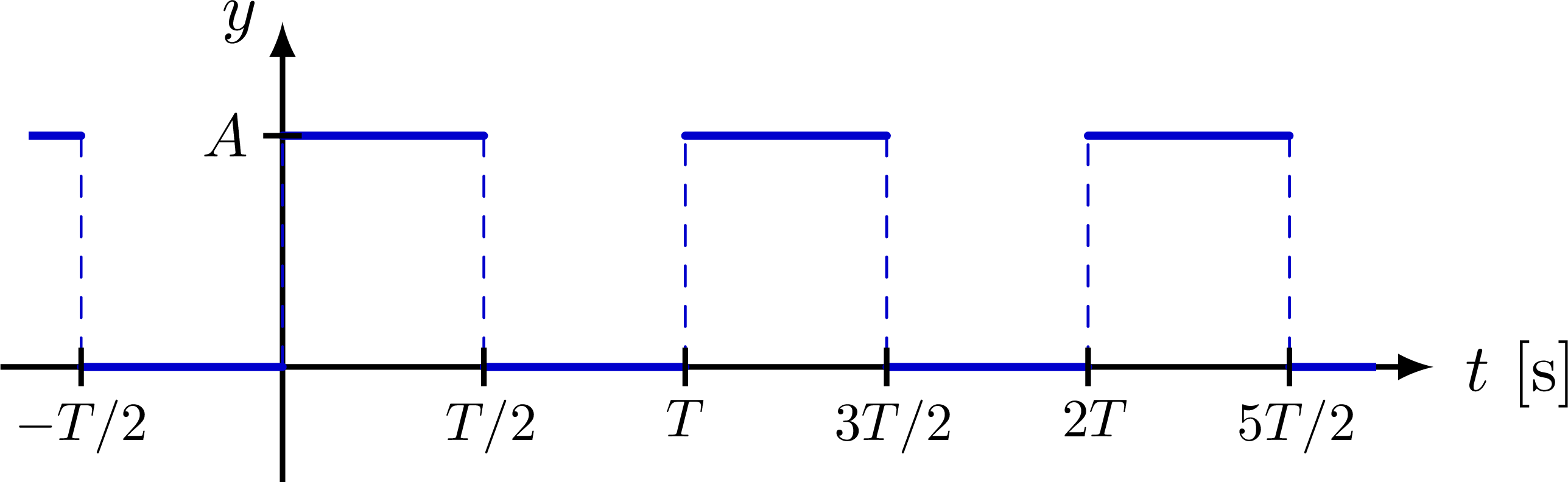
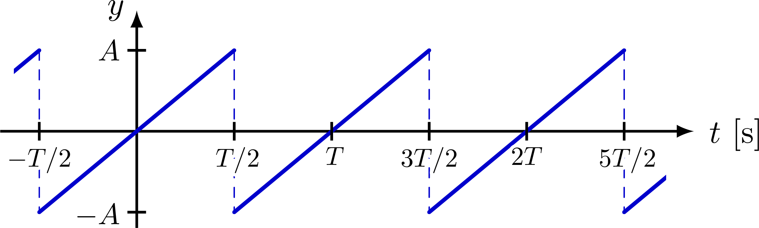
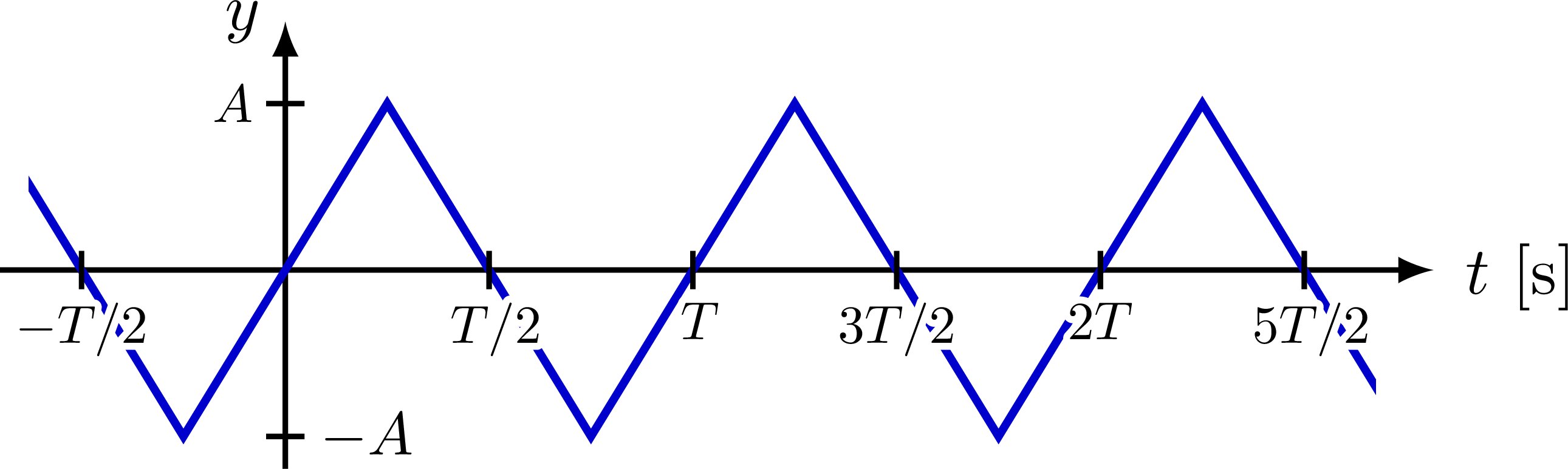
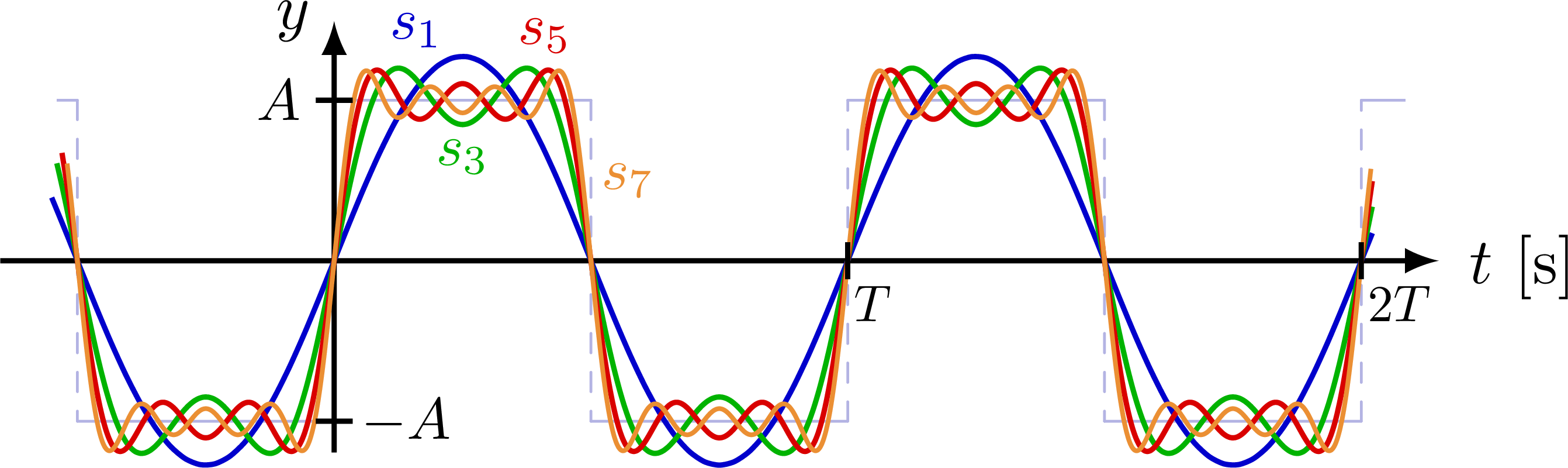
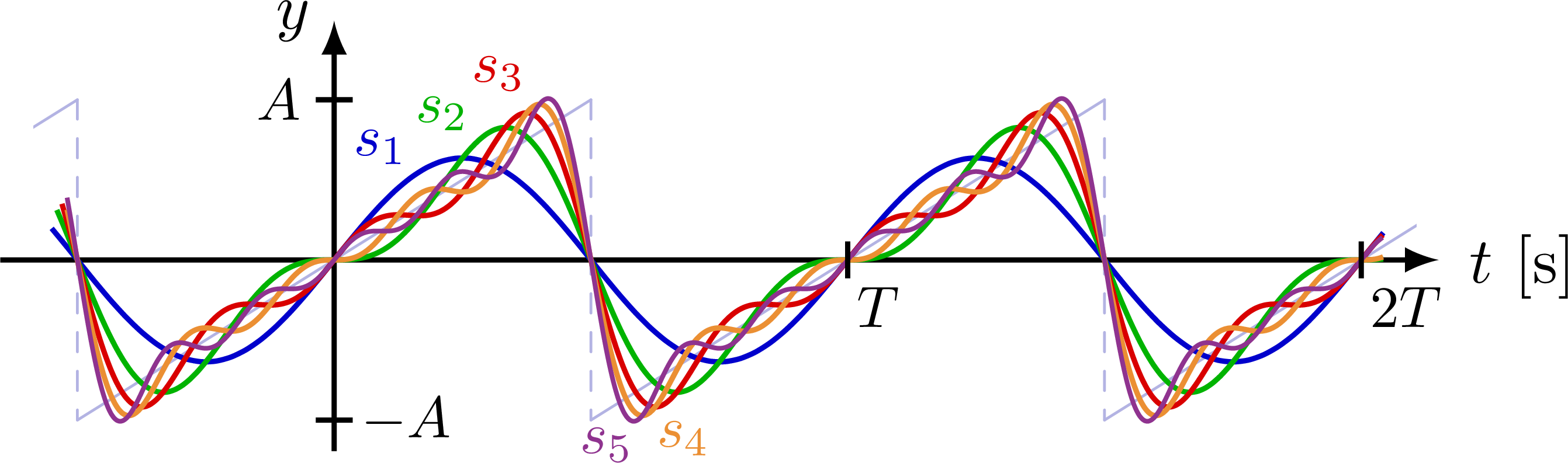
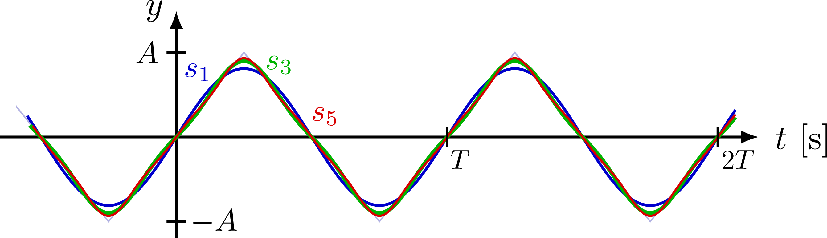
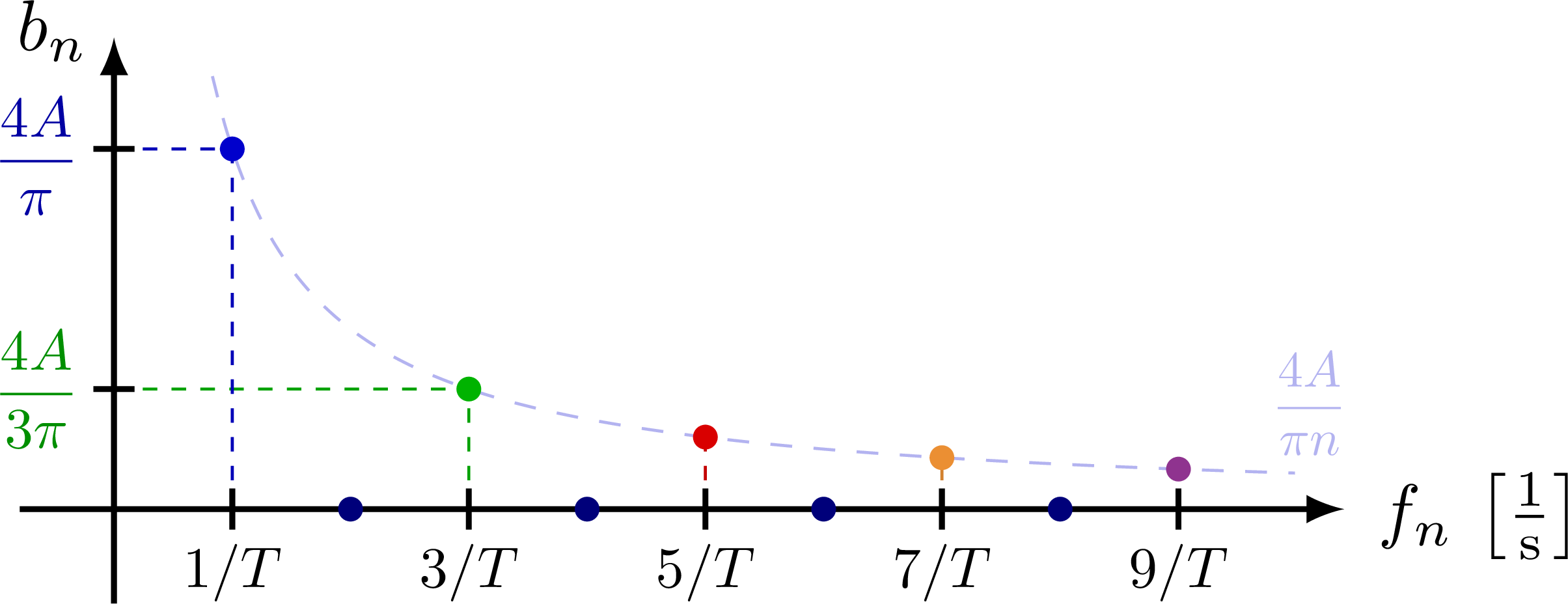
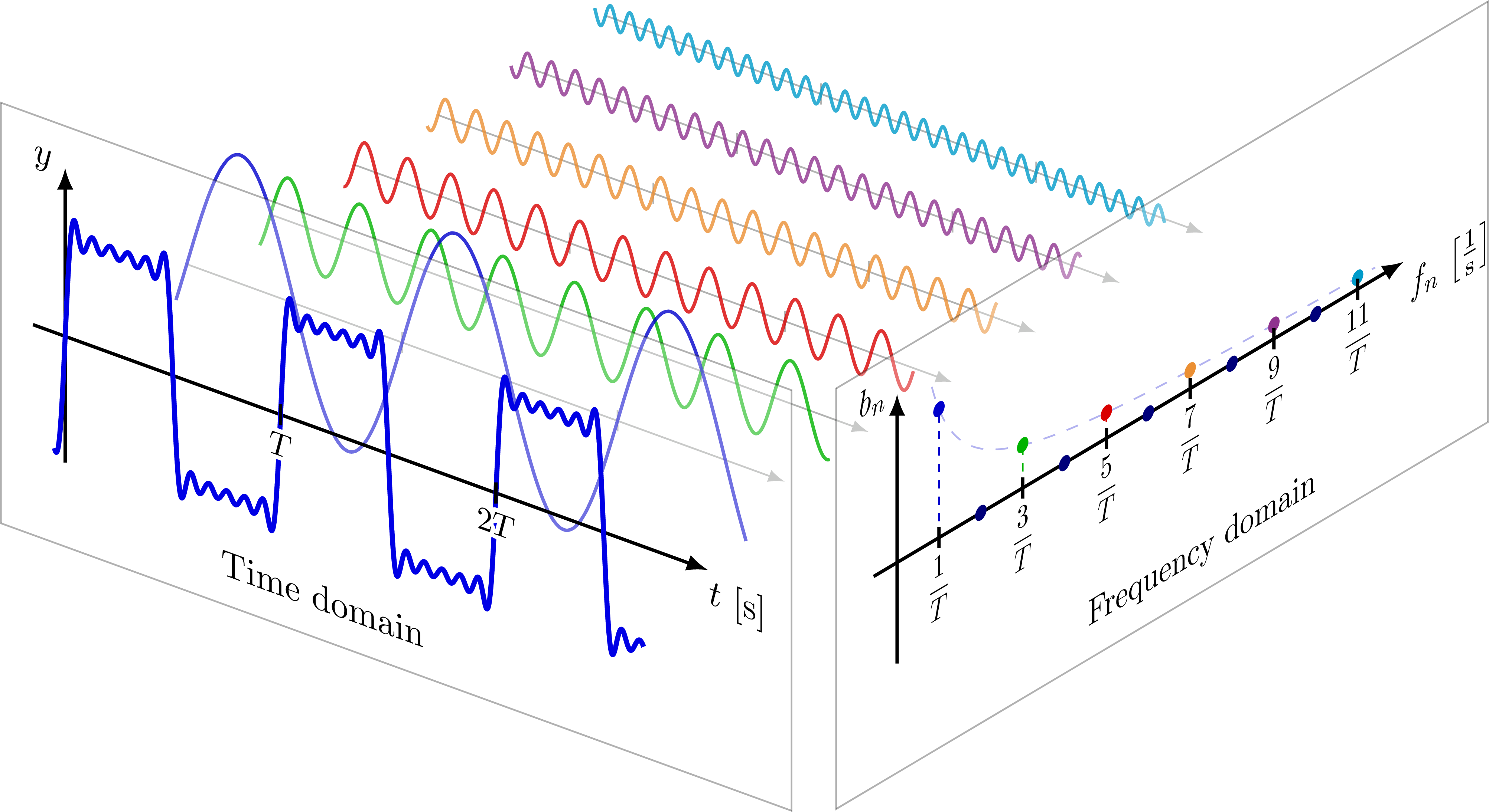
Some basic examples of Fourier series, synthesis and series of sines, cosines, rectangle, sawtooth, triangle functions, as well as a 3D figure to breakdown synthesis into the time and frequency domain.
For more Fourier analysis figures, please see the “fourier analysis” tag. These figures are used in Ben Kilminster’s lecture notes for PHY111.

Edit and compile if you like:
% Author: Izaak Neutelings (January 2021)
% http://pgfplots.net/tikz/examples/fourier-transform/
% https://tex.stackexchange.com/questions/127375/replicate-the-fourier-transform-time-frequency-domains-correspondence-illustrati
% https://www.dspguide.com/ch13/4.htm
\documentclass[border=3pt,tikz]{standalone}
\usepackage{amsmath}
\usepackage{tikz}
\usepackage{physics}
\usepackage[outline]{contour} % glow around text
\usepackage{xcolor}
\usetikzlibrary{intersections}
\usetikzlibrary{decorations.markings}
\usetikzlibrary{angles,quotes} % for pic
\usetikzlibrary{calc}
\usetikzlibrary{3d}
\contourlength{1.3pt}

\tikzset{>=latex} % for LaTeX arrow head
\colorlet{myred}{red!85!black}
\colorlet{myblue}{blue!80!black}
\colorlet{mycyan}{cyan!80!black}
\colorlet{mygreen}{green!70!black}
\colorlet{myorange}{orange!90!black!80}
\colorlet{mypurple}{red!50!blue!90!black!80}
\colorlet{mydarkred}{myred!80!black}
\colorlet{mydarkblue}{myblue!80!black}
\tikzstyle{xline}=[myblue,thick]
\def\tick#1#2{\draw[thick] (#1) ++ (#2:0.1) --++ (#2-180:0.2)}
\tikzstyle{myarr}=[myblue!50,-{Latex[length=3,width=2]}]
\def\N{90}

\begin{document}


% SQUARE WAVE
\def\xmin{-0.7*\T}   % min x axis
\def\xmax{6.0}       % max x axis
\def\ymin{-1.04}     % min y axis
\def\ymax{1.3}       % max y axis
\def\A{0.67*\ymax}   % amplitude
\def\T{(0.35*\xmax)} % period
\def\f#1{\A*4/pi/(#1)*sin(360/\T*#1*Mod(\t,\T))} %Mod(360*#1*\t/\T,360)
\begin{tikzpicture}
  \message{^^JSquare wave}

  % AXIS
  \draw[->,thick] (0,\ymin) -- (0,\ymax) node[left] {$y$};
  \draw[->,thick] ({\xmin},0) -- (\xmax,0) node[below=1,right=1] {$t$ [s]};

  % PLOT
  \begin{scope}
    \clip ({0.9*\xmin},-1.1*\A) rectangle (0.95*\xmax,1.1*\A);
    \foreach \i [evaluate={\x=\i*\T/2;}] in {-2,...,5}{
      %\coordinate (A\i) at (\x,{-\A});
      %\coordinate (B\i) at (\x,{-\A});
      \ifodd\i
        \draw[xline,very thick,line cap=round] (\x,{-\A}) --++ ({\T/2},0);
        \draw[xline,dashed,thin,line cap=round]
          ({\x+\T/2},{-\A}) --++ (0,2*\A);
      \else
        \draw[xline,very thick,line cap=round] (\x,{\A}) --++ ({\T/2},0);
        \draw[xline,dashed,thin,line cap=round]
          ({\x+\T/2},{\A}) --++ (0,-2*\A);
      \fi
    }
  \end{scope}

  % TICKS
  \tick{{ -\T/2},0}{90} node[below=-1,scale=0.8] {\contour{white}{$-T/2$}};
  \tick{{  \T  },0}{90} node[below=-1,scale=0.8] {\contour{white}{$T$}};
  \tick{{  \T/2},0}{90} node[right=1,below=-1,scale=0.8] {\contour{white}{$T/2$}};
  \tick{{3*\T/2},0}{90} node[right=1,below=-1,scale=0.8] {\contour{white}{$3T/2$}};
  \tick{{2*\T  },0}{90} node[right=1,below=-1,scale=0.8] {\contour{white}{$2T$}};
  \tick{{5*\T/2},0}{90} node[right=1,below=-1,scale=0.8] {\contour{white}{$5T/2$}};
  \tick{0,{ \A}}{  0} node[left=-1,scale=0.9] {$A$};
  \tick{0,{-\A}}{180} node[right=-2,scale=0.9] {$-A$};

\end{tikzpicture}


% SQUARE WAVE - offset
\begin{tikzpicture}
  \message{^^JSquare wave}
  \def\ymin{-0.6} % min y axis
  \def\ymax{ 1.8} % max y axis

  % AXIS
  \draw[->,thick] (0,\ymin) -- (0,\ymax) node[left] {$y$};
  \draw[->,thick] ({\xmin},0) -- (\xmax,0) node[below=1,right=1] {$t$ [s]};

  % PLOT
  \begin{scope}
    \clip ({0.9*\xmin},1.1*\ymin) rectangle (0.95*\xmax,1.1*\A);
    \foreach \i [evaluate={\x=\i*\T/2;}] in {-2,...,5}{
      \ifodd\i
        \draw[xline,very thick,line cap=round] (\x,{0}) --++ ({\T/2},0);
        \draw[xline,dashed,thin,line cap=round]
          ({\x+\T/2},{0}) --++ (0,\A);
      \else
        \draw[xline,very thick,line cap=round] (\x,{\A}) --++ ({\T/2},0);
        \draw[xline,dashed,thin,line cap=round]
          ({\x+\T/2},{\A}) --++ (0,-\A);
      \fi
    }
  \end{scope}

  % TICKS
  \tick{{ -\T/2},0}{90} node[below=-1,scale=0.8] {\contour{white}{$-T/2$}};
  \tick{{  \T  },0}{90} node[below=-1,scale=0.8] {\contour{white}{$T$}};
  \tick{{  \T/2},0}{90} node[right=1,below=-1,scale=0.8] {\contour{white}{$T/2$}};
  \tick{{3*\T/2},0}{90} node[right=1,below=-1,scale=0.8] {\contour{white}{$3T/2$}};
  \tick{{2*\T  },0}{90} node[right=1,below=-1,scale=0.8] {\contour{white}{$2T$}};
  \tick{{5*\T/2},0}{90} node[right=1,below=-1,scale=0.8] {\contour{white}{$5T/2$}};
  \tick{0,{ \A}}{  0} node[left=-1,scale=0.9] {$A$};

\end{tikzpicture}


% SAW-TOOTH WAVE
\begin{tikzpicture}
  \message{^^JSaw-tooth wave}

  % AXIS
  \draw[->,thick] (0,\ymin) -- (0,\ymax) node[left] {$y$};
  \draw[->,thick] ({\xmin},0) -- (\xmax,0) node[below=1,right=1] {$t$ [s]};

  % PLOT
  \begin{scope}
    \clip ({0.9*\xmin},-1.1*\A) rectangle (0.95*\xmax,1.1*\A);
    \foreach \i [evaluate={\x=\i*\T-\T/2;}] in {-2,...,4}{
      \draw[xline,dashed,thin,line cap=round]
        ({\x+\T},\A) --++ (0,-2*\A);
      \draw[xline,very thick,line cap=round]
        (\x,-\A) --++ ({\T},2*\A);
    }
  \end{scope}

  % TICKS
  \tick{{ -\T/2},0}{90} node[below=-1,scale=0.8] {\contour{white}{$-T/2$}};
  \tick{{  \T  },0}{90} node[right=1,below=-1,scale=0.8] {\contour{white}{$T$}};
  \tick{{  \T/2},0}{90} node[right=1,below=-1,scale=0.8] {\contour{white}{$T/2$}};
  \tick{{3*\T/2},0}{90} node[right=0,below=-1,scale=0.8] {\contour{white}{$3T/2$}};
  \tick{{2*\T  },0}{90} node[right=0,below=-1,scale=0.8] {\contour{white}{$2T$}};
  \tick{{5*\T/2},0}{90} node[right=1,below=-1,scale=0.8] {\contour{white}{$5T/2$}};
  \tick{0,{ \A}}{0} node[left=-1,scale=0.9] {$A$};
  \tick{0,{-\A}}{0} node[below=1,left=-1,scale=0.9] {$-A$};

\end{tikzpicture}


% TRIANGLE WAVE
\begin{tikzpicture}
  \message{^^JSaw-tooth wave}
  \def\T{(0.355*\xmax)} % period

  % AXIS
  \draw[->,thick] (0,\ymin) -- (0,\ymax) node[left] {$y$};
  \draw[->,thick] ({\xmin},0) -- (\xmax,0) node[below=1,right=1] {$t$ [s]};

  % PLOT
  \begin{scope}
    \clip ({0.9*\xmin},-1.1*\A) rectangle (0.95*\xmax,1.1*\A);
    \draw[xline,very thick,line cap=round]
      \foreach \i [evaluate={\x=\i*\T;}] in {-2,...,4}{
        (\x,0) --++ ({0.25*\T},\A) --++ ({\T/2},-2*\A) --++ ({0.25*\T},\A)};
  \end{scope}

  % TICKS
  \tick{{ -\T/2},0}{90} node[below=-1,scale=0.8] {\contour{white}{$-T/2$}};
  \tick{{  \T  },0}{90} node[right=1,below=-1,scale=0.8] {\contour{white}{$T$}};
  \tick{{  \T/2},0}{90} node[right=1,below=-1,scale=0.8] {\contour{white}{$T/2$}};
  \tick{{3*\T/2},0}{90} node[right=0,below=-1,scale=0.8] {\contour{white}{$3T/2$}};
  \tick{{2*\T  },0}{90} node[right=0,below=-1,scale=0.8] {\contour{white}{$2T$}};
  \tick{{5*\T/2},0}{90} node[right=1,below=-1,scale=0.8] {\contour{white}{$5T/2$}};
  \tick{0,{ \A}}{0} node[left=-1,scale=0.8] {$A$};
  \tick{0,{-\A}}{180} node[below=0,right=-1,scale=0.9] {$-A$};
  %\tick{0,{-\A}}{0} node[below=2,left=-1,scale=0.9] {$-A$};

\end{tikzpicture}


% SQUARE WAVE SYNTHESIS - time domain
\begin{tikzpicture}
   \message{^^JSquare wave synthesis - time}
   \def\xmin{-0.65*\T}  % max x axis
   \def\T{(0.465*\xmax)} % period

  % SQUARE WAVE
  \begin{scope}
    \clip ({-0.54*\T},-1.1*\A) rectangle (0.97*\xmax,1.1*\A);
    \foreach \i [evaluate={\x=\i*\T/2;}] in {-2,...,4}{
      \ifodd\i
        \draw[myblue!80!black!30,line cap=round] (\x,{-\A}) --++ ({\T/2},0);
        \draw[myblue!80!black!30,dashed,thin,line cap=round]
          ({\x+\T/2},{-\A}) --++ (0,2*\A);
      \else
        \draw[myblue!80!black!30,line cap=round] (\x,{\A}) --++ ({\T/2},0);
        \draw[myblue!80!black!30,dashed,thin,line cap=round]
          ({\x+\T/2},{\A}) --++ (0,-2*\A);
      \fi
    }
  \end{scope}

  % AXIS
  \draw[->,thick] (0,\ymin) -- (0,\ymax) node[left] {$y$};
  \draw[->,thick] ({\xmin},0) -- (\xmax,0) node[below=1,right=1] {$t$ [s]};

  % PLOT
  \draw[xline,samples=\N,smooth,variable=\t,domain=-0.55*\T:0.94*\xmax]
    plot(\t,{\f{1}});% node[pos=0.3,above] {$n=1$};
  \draw[xline,mygreen,samples=3*\N,smooth,variable=\t,domain=-0.54*\T:0.94*\xmax]
    plot(\t,{\f{1}+\f{3}});
  \draw[xline,myred,samples=5*\N,smooth,variable=\t,domain=-0.53*\T:0.94*\xmax]
    plot(\t,{\f{1}+\f{3}+\f{5}});
  \draw[xline,myorange,line width=0.7,samples=7*\N,smooth,variable=\t,domain=-0.52*\T:0.94*\xmax]
    plot(\t,{\f{1}+\f{3}+\f{5}+\f{7}});
  %\draw[xline,mypurple,samples=9*\N,smooth,variable=\t,domain=-0.52*\T:0.95*\xmax]
  %  plot(\t,{\f{1}+\f{3}+\f{5}+\f{7}+\f{9}});
  %\node[xcol,above=2,right=4] at ({720/\om},\A) {$x(t)=A\cos(\omega t)$};

  % NUMBERS
  \node[myblue,  above,scale=0.9] at ({0.16*\T},1.20*\A) {$s_1$};
  \node[mygreen, below,scale=0.9] at ({0.25*\T},0.88*\A) {$s_3$};
  \node[myred,   above,scale=0.9] at ({0.41*\T},1.17*\A) {$s_5$};
  \node[myorange,right,scale=0.9] at ({0.48*\T},0.50*\A) {$s_7$};

  % TICKS
  \tick{{  \T},0}{90} node[below right=-2,scale=0.8] {$T$};
  \tick{{2*\T},0}{90} node[below right=-2,scale=0.8] {$2T$};
  %\tick{{2*\T  },0}{90} node[right=1,below=-1,scale=0.8] {\contour{white}{$2T$}};
  \tick{0,{ \A}}{  0} node[left=-1,scale=0.9] {$A$};
  \tick{0,{-\A}}{180} node[right=-2,scale=0.9] {$-A$};

\end{tikzpicture}


% SAWTOOTH WAVE SYNTHESIS - time domain
\begin{tikzpicture}
   \message{^^JSawtooth wave synthesis - time}
   \def\xmin{-0.65*\T}  % max x axis
   \def\T{(0.465*\xmax)} % period
   \def\f#1{\A*2/pi/(#1)*(-1)^(#1-1)*sin(360/\T*#1*Mod(\t,\T))} %Mod(360*#1*\t/\T,360)

  % PLOT
  \begin{scope}
    \clip ({0.9*\xmin},-1.1*\A) rectangle (0.98*\xmax,1.1*\A);
    \foreach \i [evaluate={\x=\i*\T-\T/2;}] in {-2,...,4}{
      \draw[myblue!80!black!30,line cap=round]
        (\x,-\A) --++ ({\T},2*\A);
      \draw[myblue!80!black!30,dashed,thin,line cap=round]
        ({\x+\T},\A) --++ (0,-2*\A);
    }
  \end{scope}

  % AXIS
  \draw[->,thick] (0,\ymin) -- (0,\ymax) node[left] {$y$};
  \draw[->,thick] ({\xmin},0) -- (\xmax,0) node[below=1,right=1] {$t$ [s]};

  % PLOT
  \draw[xline,samples=\N,smooth,variable=\t,domain=-0.55*\T:0.95*\xmax]
    plot(\t,{\f{1}});% node[pos=0.3,above] {$n=1$};
  \draw[xline,mygreen,samples=2*\N,smooth,variable=\t,domain=-0.54*\T:0.95*\xmax]
    plot(\t,{\f{1}+\f{2}});
  \draw[xline,myred,samples=3*\N,smooth,variable=\t,domain=-0.53*\T:0.95*\xmax]
    plot(\t,{\f{1}+\f{2}+\f{3}});
  \draw[xline,myorange,samples=4*\N,smooth,variable=\t,domain=-0.52*\T:0.95*\xmax]
    plot(\t,{\f{1}+\f{2}+\f{3}+\f{4}});
  \draw[xline,mypurple,line width=0.7,samples=5*\N,smooth,variable=\t,domain=-0.52*\T:0.95*\xmax]
    plot(\t,{\f{1}+\f{2}+\f{3}+\f{4}+\f{5}});

  % NUMBERS
  \node[myblue,  above,scale=0.9] at ({0.09*\T}, 0.47*\A) {$s_1$};
  \node[mygreen, above,scale=0.9] at ({0.21*\T}, 0.68*\A) {$s_2$};
  \node[myred,   above,scale=0.9] at ({0.32*\T}, 0.93*\A) {$s_3$};
  \node[myorange,below,scale=0.9] at ({0.68*\T},-0.88*\A) {$s_4$};
  \node[mypurple,below,scale=0.9] at ({0.53*\T},-0.92*\A) {$s_5$};

  % TICKS
  \tick{{  \T},0}{90} node[below right=-2,scale=0.9] {$T$};
  \tick{{2*\T},0}{90} node[below right=-2,scale=0.9] {$2T$};
  \tick{0,{ \A}}{  0} node[left=-1,scale=0.9] {$A$};
  \tick{0,{-\A}}{180} node[right=-2,scale=0.9] {$-A$};

\end{tikzpicture}


% TRIANGLE WAVE SYNTHESIS - time domain
\begin{tikzpicture}
  \message{^^JTriangle wave synthesis - time}
   \def\xmin{-0.65*\T}  % max x axis
   \def\T{(0.465*\xmax)} % period
   \def\f#1{\A*8/pi^2/(#1)^2*(-1)^((#1-1)/2)*sin(360/\T*#1*Mod(\t,\T))} %Mod(360*#1*\t/\T,360)

  % SQUARE WAVE
  \begin{scope}
    \clip ({-0.59*\T},-1.1*\A) rectangle (0.96*\xmax,1.1*\A);
    \draw[myblue!80!black!30,line cap=round]
      \foreach \i [evaluate={\x=\i*\T;}] in {-2,...,4}{
        (\x,0) --++ ({0.25*\T},\A) --++ ({\T/2},-2*\A) --++ ({0.25*\T},\A)};
  \end{scope}

  % AXIS
  \draw[->,thick] (0,\ymin) -- (0,\ymax) node[left] {$y$};
  \draw[->,thick] ({\xmin},0) -- (\xmax,0) node[below=1,right=1] {$t$ [s]};

  % PLOT
  \draw[xline,samples=\N,smooth,variable=\t,domain=-0.55*\T:0.96*\xmax]
    plot(\t,{\f{1}});% node[pos=0.3,above] {$n=1$};
  \draw[xline,mygreen,line width=1.2,samples=2*\N,smooth,variable=\t,domain=-0.54*\T:0.96*\xmax]
    plot(\t,{\f{1}+\f{3}});
  \draw[xline,myred,line width=0.6,samples=3*\N,smooth,variable=\t,domain=-0.53*\T:0.96*\xmax]
    plot(\t,{\f{1}+\f{3}+\f{5}});
  %\draw[xline,myorange,line width=0.6,samples=3*\N,smooth,variable=\t,domain=-0.52*\T:0.96*\xmax]
  %  plot(\t,{\f{1}+\f{3}+\f{5}+\f{7}});
  %\draw[xline,mypurple,samples=9*\N,smooth,variable=\t,domain=-0.52*\T:0.95*\xmax]
  %  plot(\t,{\f{1}+\f{3}+\f{5}+\f{7}+\f{9}});
  %\node[xcol,above=2,right=4] at ({720/\om},\A) {$x(t)=A\cos(\omega t)$};

  % NUMBERS
  \node[myblue,  above,scale=0.9] at ({0.08*\T},0.53*\A) {$s_1$};
  \node[mygreen, above,scale=0.9] at ({0.38*\T},0.62*\A) {$s_3$};
  \node[myred,   above,scale=0.9] at ({0.55*\T},0.01*\A) {$s_5$};
  %\node[myorange,right,scale=0.9] at ({0.50*\T},0.55*\A) {$s_7$};

  % TICKS
  \tick{{  \T},0}{90} node[below right=-2,scale=0.8] {$T$};
  \tick{{2*\T},0}{90} node[below right=-2,scale=0.8] {$2T$};
  %\tick{{2*\T  },0}{90} node[right=1,below=-1,scale=0.8] {\contour{white}{$2T$}};
  \tick{0,{ \A}}{  0} node[left=-1,scale=0.9] {$A$};
  \tick{0,{-\A}}{180} node[right=-2,scale=0.9] {$-A$};

\end{tikzpicture}


%% SQUARE WAVE SYNTHESIS - relative difference
%\begin{tikzpicture}
%  \message{^^JSquare wave synthesis - relative difference}
%  \def\xmin{-0.60*\T} % min x axis
%  \def\ymin{-1.2}     % min y axis
%  \def\ymax{1.4}      % max y axis
%  \def\T{(0.6*\xmax)} % period
%
%  % AXIS
%  \draw[->,thick] (0,\ymin) -- (0,\ymax) node[left] {$y$};
%  \draw[->,thick] ({\xmin},0) -- (\xmax,0) node[below=1,right=1] {$t$ [s]};
%
%  % PLOT
%  \foreach \i [evaluate={\x=\i*\T/2;}] in {-1,...,2}{
%    \draw[xline,samples=\N,smooth,variable=\t,domain=\x:\x+\T/2]
%      plot(\t,{(\f{1}-((-1)^\i)*\A)/abs(\A)});
%    \draw[xline,mygreen,samples=\N,smooth,variable=\t,domain=\x:\x+\T/2]
%      plot(\t,{(\f{1}+\f{3}-((-1)^\i)*\A)/abs(\A)});
%    \draw[xline,myred,samples=\N,smooth,variable=\t,domain=\x:\x+\T/2]
%      plot(\t,{(\f{1}+\f{3}+\f{5}-((-1)^\i)*\A)/abs(\A)});
%    \draw[xline,myorange,samples=\N,smooth,variable=\t,domain=\x:\x+\T/2]
%      plot(\t,{(\f{1}+\f{3}+\f{5}+\f{7}-((-1)^\i)*\A)/abs(\A)});
%    \draw[xline,mypurple,samples=\N,smooth,variable=\t,domain=\x:\x+\T/2]
%      plot(\t,{(\f{1}+\f{3}+\f{5}+\f{7}+\f{9}-((-1)^\i)*\A)/abs(\A)});
%  }
%
%%  % NUMBERS
%%  \node[myblue,  above,scale=0.7] at ({0.19*\T},1.25*\A) {$n=1$};
%%  \node[mygreen, below,scale=0.7] at ({0.25*\T},0.90*\A) {$n=2$};
%%  \node[myred,   above,scale=0.7] at ({0.51*\T},1.21*\A) {$n=3$};
%%  \node[myorange,right,scale=0.7] at ({0.50*\T},0.55*\A) {$n=4$};
%
%  % TICKS
%  \tick{{  \T},0}{90} node[below right=-2,scale=0.8] {$T$};
%  \tick{{2*\T},0}{90} node[below right=-2,scale=0.8] {$2T$};
%  %\tick{{2*\T  },0}{90} node[right=1,below=-1,scale=0.8] {\contour{white}{$2T$}};
%  \tick{0,{ \A}}{  0} node[left=-1,scale=0.8] {$A$};
%  %\tick{0,{-\A}}{180} node[right=-2,scale=0.8] {$-A$};
%
%\end{tikzpicture}


% SQUARE WAVE SYNTHESIS - frequency domain
\begin{tikzpicture}
  \message{^^JSquare wave synthesis - frequency}
  \def\ymax{2.3}     % max y axis
  \def\A{0.6*\ymax}  % amplitude
  \def\w{\xmax/10.4} % component spacing

  % AXIS
  \draw[->,thick] (0,-0.2*\ymax) -- (0,\ymax) node[above=1,left] {$b_n$};
  \draw[->,thick] ({-0.2*\ymax},0) -- (\xmax,0)
    node[below=1,right=1] {$f_n$ $\left[\frac{1}{\mathrm{s}}\right]$};
  \draw[myblue!90!black,dash pattern=on 2 off 2] (0,{\A*4/pi}) --++ ({\w},0);
  \draw[mygreen!90!black,dash pattern=on 2 off 2] (0,{\A*4/3/pi}) --++ ({3*\w},0);

  % ENVELOPE
  \draw[myblue!30,dashed,samples=\N,smooth,variable=\t,domain=0.08*\xmax:0.96*\xmax]
    plot(\t,{\A*4/pi/\t*\w}) node[right=2,above=0,scale=0.7] {$\dfrac{4A}{\pi n}$};

  % COMPONENTS
  \foreach \i/\col [evaluate={\x=\w*\i;}] in {
      1/myblue,3/mygreen,5/myred,7/myorange,9/mypurple}{
    \draw[\col!90!black,dash pattern=on 2 off 2]
      (\x,0) --++ (0,{\A*4/pi/\i});
    \fill[\col] (\x,{\A*4/pi/\i}) circle(0.06);
    \tick{\x,0}{90}
      node[below=-1,scale=0.8]
      {$\i/T$};
      %{$\dfrac{\i}{T}$}; %f_\i=\ifnum\i=1 \else \i \fi T
  }
  \foreach \i/\col [evaluate={\x=\w*\i;}] in {2,4,...,8}{
    \fill[myblue!60!black] (\x,0) circle(0.06);
  }
  \tick{0,\A*4/pi}{0} node[myblue!80!black,below=1,left=-1,scale=0.8] {$\dfrac{4A}{\pi}$};
  \tick{0,\A*4/3/pi}{0} node[mygreen!80!black,below=0,left=-1,scale=0.8] {$\dfrac{4A}{3\pi}$};

\end{tikzpicture}


% SAWTOOTH WAVE SYNTHESIS - frequency domain
% https://mathworld.wolfram.com/FourierSeriesSawtoothWave.html
\begin{tikzpicture}
  \message{^^JSquare wave synthesis - frequency}
  \def\ymin{-1.6}    % min y axis
  \def\ymax{2.3}     % max y axis
  \def\A{1.18*\ymax} % amplitude
  \def\w{\xmax/7}    % component spacing

  % AXIS
  \draw[->,thick] (0,\ymin) -- (0,\ymax) node[above=1,left] {$b_n$};
  \draw[->,thick] ({-0.2*\ymax},0) -- (\xmax,0)
    node[below=1,right=1] {$f_n$ $\left[\frac{1}{\mathrm{s}}\right]$};
  \draw[myblue!90!black,dash pattern=on 2 off 2] (0,{\A*2/pi}) --++ ({\w},0);
  \draw[mygreen!90!black,dash pattern=on 2 off 2] (0,{-\A/pi}) --++ ({2*\w},0);

  % ENVELOPE
  \draw[myblue!30,dashed,samples=\N,smooth,variable=\t,domain=0.115*\xmax:0.96*\xmax]
    plot(\t,{\A*2/pi/\t*\w}) node[right=2,above=0,scale=0.7] {$\dfrac{2A}{\pi n}$};
  \draw[myblue!30,dashed,samples=\N,smooth,variable=\t,domain=0.166*\xmax:0.96*\xmax]
    plot(\t,{-\A*2/pi/\t*\w}) node[left=1,below=0,scale=0.7] {$-\dfrac{2A}{\pi n}$};

  % COMPONENTS
  \foreach \i/\col [evaluate={\x=\w*\i;}] in {
      1/myblue,2/mygreen,3/myred,4/myorange,5/mypurple,6/mycyan}{
    \ifodd\i
      \draw[\col!90!black,dash pattern=on 2 off 2]
        (\x,0) --++ (0,{\A*2/pi/\i});
      \fill[\col] (\x,{\A*2/pi/\i}) circle(0.06);
      \tick{\x,0}{90} node[below=-1,scale=0.8] {\contour{white}{$\i/T$}};
    \else
      \draw[\col!90!black,dash pattern=on 2 off 2]
        (\x,0) --++ (0,{-\A*2/pi/\i});
      \fill[\col] (\x,{-\A*2/pi/\i}) circle(0.06);
      \tick{\x,0}{-90} node[above=-1,scale=0.8] {\contour{white}{$\i/T$}};
    \fi
  }
  \tick{0,\A*2/pi}{0} node[myblue!80!black,below=1,left=-1,scale=0.8] {$\dfrac{2A}{\pi}$};
  \tick{0,-\A/pi}{0} node[mygreen!80!black,below=0,left=-1,scale=0.8] {$-\dfrac{A}{\pi}$};

\end{tikzpicture}


% TRIANGLE WAVE SYNTHESIS - frequency domain
% https://archive.lib.msu.edu/crcmath/math/math/f/f270.htm
% https://mathworld.wolfram.com/FourierSeriesTriangleWave.html
\begin{tikzpicture}
  \message{^^JTriangle wave synthesis - frequency}
  \def\ymin{-1.0}    % min y axis
  \def\ymax{2.9}     % max y axis
  \def\A{1.05*\ymax} % amplitude
  \def\w{\xmax/9.1}  % component spacing

  % AXIS
  \draw[->,thick] (0,\ymin) -- (0,\ymax) node[above=1,left] {$b_n$};
  \draw[->,thick] ({-0.2*\ymax},0) -- (\xmax,0)
    node[below=1,right=1] {$f_n$ $\left[\frac{1}{\mathrm{s}}\right]$};
  \draw[myblue!90!black,dash pattern=on 2 off 2] (0,{8*\A/pi^2}) --++ ({\w},0);
  \draw[mygreen!90!black,dash pattern=on 2 off 2] (0,{-8*\A/pi^2/9}) --++ ({3*\w},0);

  % ENVELOPE
  \draw[myblue!30,dashed,samples=\N,smooth,variable=\t,domain=0.10*\xmax:0.96*\xmax]
    plot(\t,{ 8*\A*(\w/pi/\t)^2}) node[left=2,above=0,scale=0.7] {$\dfrac{8A}{\pi^2 n^2}$};
  \draw[myblue!30,dashed,samples=\N,smooth,variable=\t,domain=0.18*\xmax:0.96*\xmax]
    plot(\t,{-8*\A*(\w/pi/\t)^2}) node[left=5,below=0,scale=0.7] {$-\dfrac{8A}{\pi^2 n^2}$};

  % COMPONENTS
  \foreach \i/\col [evaluate={\x=\w*\i;}] in {
    1/myblue,3/mygreen,5/myred,7/myorange}{ %,9/mypurple,11/mycyan
    \draw[\col!90!black,dash pattern=on 2 off 2]
      (\x,0) --++ (0,{8*\A/(pi^2)/(\i^2)*(-1)^((\i-1)/2)});
    \fill[\col] (\x,{8*\A/(pi^2)/(\i^2)*(-1)^((\i-1)/2)}) circle(0.06);
    \ifnum\i=3
      \tick{\x,0}{90} node[below=4,scale=0.8] {$\i/T$}; %{\contour{white}{$\i/T$}};
    \else
      \tick{\x,0}{90} node[below=-1,scale=0.8] {\contour{white}{$\i/T$}};
    \fi
  }
  \foreach \i/\col [evaluate={\x=\w*\i;}] in {2,4,...,8}{
    \fill[myblue!60!black] (\x,0) circle(0.06);
  }
  \tick{0, 8*\A/pi^2  }{0} node[myblue!80!black,below=5,left=-1,scale=0.8] {$\dfrac{8A}{\pi^2}$};
  \tick{0,-8*\A/pi^2/9}{0} node[mygreen!80!black,below=6,left=-1,scale=0.8] {$-\dfrac{8A}{9\pi^2}$};

\end{tikzpicture}


% SYNTHESIS 3D
\begin{tikzpicture}[x=(-20:0.9), y=(90:0.9), z=(42:1.1)]
  \message{^^JSynthesis 3D}
  \def\xmax{6.5}        % max x axis
  \def\ymin{-1.2}       % min y axis
  \def\ymax{1.6}        % max y axis
  \def\zmax{5.8}        % max z axis
  \def\xf{1.17*\xmax}   % x position frequency axis
  \def\A{(0.60*\ymax)}  % amplitude
  \def\T{(0.335*\xmax)} % period
  \def\w{\zmax/11.2}    % spacing components

  % COMPONENTS
  \foreach \i/\col [evaluate={\z=\w*\i;}] in {
      11/mycyan,9/mypurple,7/myorange,5/myred,3/mygreen,1/myblue}{
    \draw[black!30] ({\T},0.1,\z) --++ (0,-0.2,0);
    \draw[black!30] ({2*\T},0.1,\z) --++ (0,-0.2,0);
    \draw[->,black!30] (0,0,\z) --++ (0.93*\xmax,0,0);
    \draw[xline,\col,opacity=0.8,thick,
          samples=\i*\N,smooth,variable=\t,domain=-0.05*\T:0.87*\xmax]
      plot(\t,{\f{\i}},\z);
  }

  % TIME DOMAIN
  \begin{scope}[shift={(0,0,-0.17*\zmax)}]
    \draw[black,fill=white,opacity=0.3,canvas is xy plane at z=0]
      (-0.1*\xmax,-1.25*\ymax) rectangle (1.13*\xmax,1.25*\ymax);
    \draw[->,thick] (-0.05*\xmax,0,0) -- (\xmax,0,0)
      node[below right=-3,canvas is xy plane at z=0] {$t$ [s]};
    \draw[->,thick] (0,\ymin,0) -- (0,\ymax,0)
      node[left,canvas is xy plane at z=0] {$y$};
    \draw[xline,blue!90!black,very thick,
          samples=9*\N,smooth,variable=\t,domain=-0.05*\T:0.9*\xmax]
      plot(\t,{\f{1}+\f{3}+\f{5}+\f{7}+\f{9}+\f{11}},0); %node[above] {$f$};
    \tick{{\T},0,0}{90}
      node[below=-1,scale=0.9,canvas is xy plane at z=0] {\contour{white}{$T$}};
    \tick{{2*\T},0,0}{90}
      node[below=-1,scale=0.9,canvas is xy plane at z=0] {\contour{white}{$2T$}};
    \node[scale=1,canvas is xy plane at z=0] at (0.4*\xmax,-\ymax,0) {Time domain};
  \end{scope}

  % FREQUENCY DOMAIN
  \begin{scope}[shift={(\xf,0,0)}]
    \draw[black,fill=white,opacity=0.3,canvas is zy plane at x=0]
      (-0.13*\zmax,-1.25*\ymax) rectangle (1.26*\zmax,1.25*\ymax);
    %\draw[->,thick] (0,0,0) -- (0,0,\zmax) node[above left=-1] {$z$};
    %\draw[->,thick] (\xmax,0,0) --++ (0,0,\zmax);
    \draw[->,thick] (0,0.8*\ymin,0) -- (0,\ymax,0)
      node[above=2,left=0,canvas is zy plane at x=0] {$b_n$};
      %node[pos=0.84,left=2,fill=white,inner sep=0] {$b_n$};
    \draw[->,thick] (0,0,-0.05*\zmax) --++ (0,0,1.13*\zmax)
      node[below right=-1,canvas is zy plane at x=0] {$f_n$ $\left[\frac{1}{\mathrm{s}}\right]$};
    \node[scale=1,canvas is zy plane at x=0] at (0,-\ymax,0.65*\zmax) {Frequency domain};
    \draw[myblue!30,dashed,samples=3*\N,smooth,variable=\t,domain=0.074*\zmax:1.02*\zmax]
      plot(0,{\A*4/pi/\t*\w},\t); %node[right=2,above=0,scale=0.7] {$\dfrac{4A}{\pi n}$};
    \foreach \i/\col [evaluate={\z=\w*\i;}] in {
        11/mycyan,9/mypurple,7/myorange,5/myred,3/mygreen,1/myblue}{
      \draw[\col,dash pattern=on 2 off 2]
        (0,0,\z) --++ (0,{\A*4/pi/\i},0);
      \fill[\col,canvas is zy plane at x=0]
        %(\xf,{\A*4/pi/\i},\z) circle(0.08);
        (\z,{\A*4/pi/\i}) circle(0.07);
      \tick{0,0,\z}{90}
        node[below=-1,scale=0.85,canvas is zy plane at x=0]
        {$\dfrac{\i}{T}$}; %f_\i=\ifnum\i=1 \else \i \fi T
    }
    \foreach \i [evaluate={\z=\w*\i;}] in {2,4,...,10}{
      \fill[myblue!60!black,canvas is zy plane at x=0] (\z,0) circle(0.07);
    }
  \end{scope}

\end{tikzpicture}


\end{document}
Click to download: fourier_series.tex • fourier_series.pdf
Open in Overleaf: fourier_series.tex


Dear Prof. Izaak Neutelings,
Your codes are fabulous. I like them. I am a beginner of Tikz. I have a question about the codes for Fourier series.
When you plot the partial sum of the series, you used codes just like this:
plot(\t,{\f{1}+\f{3}+\f{5}+\f{7}+\f{9}+\f{11}},0); %node[above] {$f$};
Can we define a function Sn(N)=f(1)+…+f(N), and use codes like this:
plot(\t,{Sn(x},0); %node[above] {$f$}; ?
Maybe I want to plot Sn(100) . It looks stupid that typing {f(1)+…+f(100}.
Since it is hopeless that you can see this, I am still looking forward to your reply.
Have a good weekend.
Harry Liu