Fourier transform

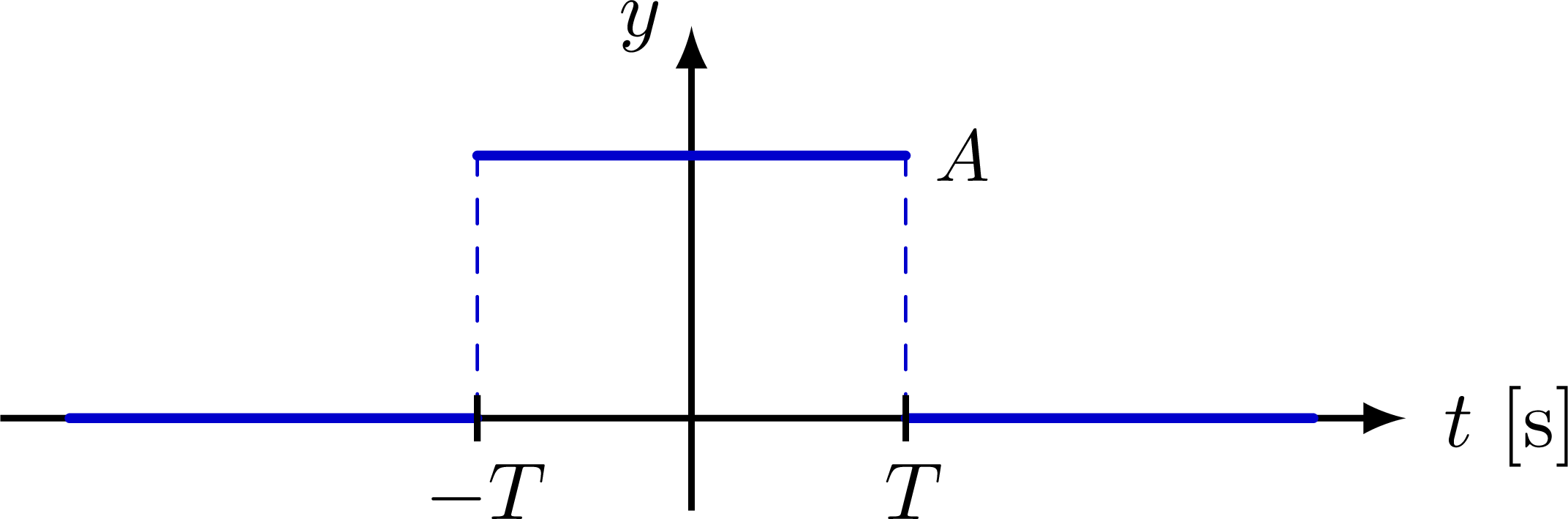
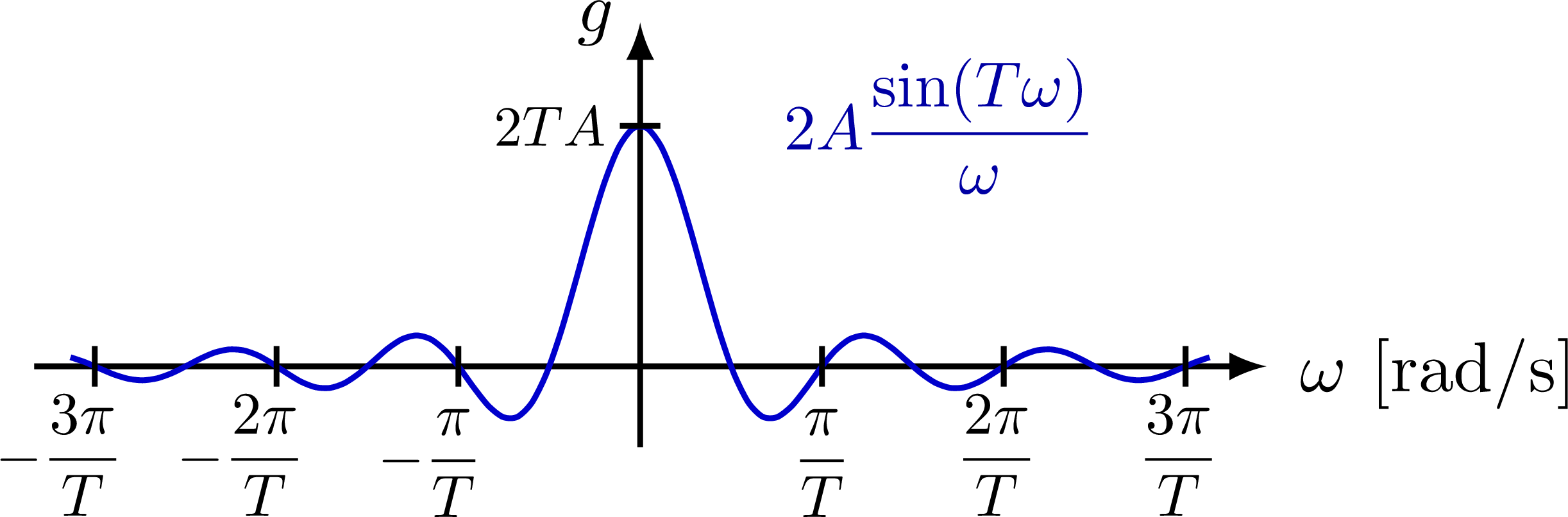
A basic examples of the Fourier transform of a rectangular function.
For more Fourier analysis figures, please see the “fourier analysis” tag. These figures are used in Ben Kilminster’s lecture notes for PHY111.

Edit and compile if you like:

% Author: Izaak Neutelings (January 2021)
% http://pgfplots.net/tikz/examples/fourier-transform/
% https://tex.stackexchange.com/questions/127375/replicate-the-fourier-transform-time-frequency-domains-correspondence-illustrati
% https://www.dspguide.com/ch13/4.htm
\documentclass[border=3pt,tikz]{standalone}
\usepackage{amsmath}
\usepackage{tikz}
\usepackage{physics}
\usepackage[outline]{contour} % glow around text
\usepackage{xcolor}
\usetikzlibrary{intersections}
\usetikzlibrary{decorations.markings}
\usetikzlibrary{angles,quotes} % for pic
\usetikzlibrary{calc}
\usetikzlibrary{3d}
\contourlength{1.3pt}

\tikzset{>=latex} % for LaTeX arrow head
\colorlet{myred}{red!85!black}
\colorlet{myblue}{blue!80!black}
\colorlet{mycyan}{cyan!80!black}
\colorlet{mygreen}{green!70!black}
\colorlet{myorange}{orange!90!black!80}
\colorlet{mypurple}{red!50!blue!90!black!80}
\colorlet{mydarkred}{myred!80!black}
\colorlet{mydarkblue}{myblue!80!black}
\tikzstyle{xline}=[myblue,thick]
\def\tick#1#2{\draw[thick] (#1) ++ (#2:0.1) --++ (#2-180:0.2)}
\tikzstyle{myarr}=[myblue!50,-{Latex[length=3,width=2]}]
\def\N{80}

\begin{document}


% RECTANGULAR FUNCTION
\def\xmin{-0.7*\T} % min x axis
\def\xmax{3.0}     % max x axis
\def\ymin{-0.4}    % min y axis
\def\ymax{1.7}     % max y axis
\def\A{0.67*\ymax} % amplitude
\def\T{0.31*\xmax} % period
\begin{tikzpicture}
  \message{^^JRectangular function}
  \draw[->,thick] (0,\ymin) -- (0,\ymax) node[left] {$y$};
  \draw[->,thick] (-\xmax,0) -- (\xmax+0.1,0) node[below=1,right=1] {$t$ [s]};
  \draw[xline,very thick,line cap=round]
    ({-\T},{\A}) -- ({\T},{\A}) node[black,right=0,scale=0.9] {$A$}
    ({-\T},0) -- ({-0.9*\xmax},0)
    ({ \T},0) -- ({0.9*\xmax},0);
  \draw[xline,dashed,thin,line cap=round]
    ({-\T},0) --++ (0,{\A})
    ({ \T},0) --++ (0,{\A});
  \tick{{ -\T},0}{90} node[right=1,below=-1,scale=1] {$-T$};
  \tick{{  \T},0}{90} node[right=1,below=-1,scale=1] {$T$};
  %\tick{0,{ \A}}{  0} node[left=-1,scale=0.9] {$A$};
\end{tikzpicture}


% RECTANGULAR FUNCTION - frequency domain
\begin{tikzpicture}
  \message{^^JRectangular function - frequency domain}
  \def\T{0.30*\xmax} % period
  \def\A{0.70*\ymax} % amplitude
  \draw[->,thick] (0,\ymin) -- (0,\ymax) node[left] {$g$};
  \draw[->,thick] (-\xmax,0) -- (\xmax+0.1,0) node[below=1,right=1] {$\omega$ [rad/s]};
  \draw[xline,samples=\N,smooth,variable=\t,domain=-0.94*\xmax:0.94*\xmax]
    plot(\t,{\A*sin(360/(\T)*\t)/(2*pi)*(\T)/\t});
  \tick{{-3*\T},0}{90} node[left=  5,below=-2,scale=0.85] {\strut$-\dfrac{3\pi}{T}$};
  \tick{{-2*\T},0}{90} node[left=  5,below=-2,scale=0.85] {\strut$-\dfrac{2\pi}{T}$};
  \tick{{  -\T},0}{90} node[left=  4,below= 0,scale=0.85] {\strut$-\dfrac{\pi}{T}$};
  \tick{{   \T},0}{90} node[right= 0,below= 0,scale=0.85] {\strut$ \dfrac{\pi}{T}$};
  \tick{{ 2*\T},0}{90} node[right=-1,below=-2,scale=0.85] {\strut$ \dfrac{2\pi}{T}$};
  \tick{{ 3*\T},0}{90} node[right=-1,below=-2,scale=0.85] {\strut$ \dfrac{3\pi}{T}$};
  \tick{0,{\A}}{0} node[left=-1,scale=0.8] {$2TA$};
  \node[mydarkblue,right,scale=0.9] at (0.2*\xmax,\A)
    {$2A\dfrac{\sin(T\omega)}{\omega}$}; %g(\omega) = 
\end{tikzpicture}


%% SYNTHESIS 3D
%\begin{tikzpicture}[x=(-20:0.9), y=(90:0.9), z=(42:1.1)]
%  \message{^^JSynthesis 3D}
%  \def\xmax{6.5}        % max x axis
%  \def\ymin{-1.2}       % min y axis
%  \def\ymax{1.6}        % max y axis
%  \def\zmax{5.8}        % max z axis
%  \def\xf{1.17*\xmax}   % x position frequency axis
%  \def\A{(0.60*\ymax)}  % amplitude
%  \def\T{(0.335*\xmax)} % period
%  \def\w{\zmax/11.2}    % spacing components
%  
%  % COMPONENTS
%  \foreach \i/\col [evaluate={\z=\w*\i;}] in {
%      11/mycyan,9/mypurple,7/myorange,5/myred,3/mygreen,1/myblue}{
%    \draw[black!30] ({\T},0.1,\z) --++ (0,-0.2,0);
%    \draw[black!30] ({2*\T},0.1,\z) --++ (0,-0.2,0);
%    \draw[->,black!30] (0,0,\z) --++ (0.93*\xmax,0,0);
%    \draw[xline,\col,opacity=0.8,thick,
%          samples=\i*\N,smooth,variable=\t,domain=-0.05*\T:0.87*\xmax]
%      plot(\t,{\f{\i}},\z);
%  }
%  
%  % TIME DOMAIN
%  \begin{scope}[shift={(0,0,-0.17*\zmax)}]
%    \draw[black,fill=white,opacity=0.3,canvas is xy plane at z=0]
%      (-0.1*\xmax,-1.25*\ymax) rectangle (1.13*\xmax,1.25*\ymax);
%    \draw[->,thick] (-0.05*\xmax,0,0) -- (\xmax,0,0)
%      node[below right=-3,canvas is xy plane at z=0] {$t$ [s]};
%    \draw[->,thick] (0,\ymin,0) -- (0,\ymax,0)
%      node[left,canvas is xy plane at z=0] {$y$};
%    \draw[xline,blue!90!black,very thick,
%          samples=9*\N,smooth,variable=\t,domain=-0.05*\T:0.9*\xmax]
%      plot(\t,{\f{1}+\f{3}+\f{5}+\f{7}+\f{9}+\f{11}},0); %node[above] {$f$};
%    \tick{{\T},0,0}{90}
%      node[below=-1,scale=0.9,canvas is xy plane at z=0] {\contour{white}{$T$}};
%    \tick{{2*\T},0,0}{90}
%      node[below=-1,scale=0.9,canvas is xy plane at z=0] {\contour{white}{$2T$}};
%    \node[scale=1,canvas is xy plane at z=0] at (0.4*\xmax,-\ymax,0) {Time domain};
%  \end{scope}
%  
%  % FREQUENCY DOMAIN
%  \begin{scope}[shift={(\xf,0,0)}]
%    \draw[black,fill=white,opacity=0.3,canvas is zy plane at x=0]
%      (-0.13*\zmax,-1.25*\ymax) rectangle (1.26*\zmax,1.25*\ymax);
%    %\draw[->,thick] (0,0,0) -- (0,0,\zmax) node[above left=-1] {$z$};
%    %\draw[->,thick] (\xmax,0,0) --++ (0,0,\zmax);
%    \draw[->,thick] (0,0.8*\ymin,0) -- (0,\ymax,0)
%      node[pos=1,left=0,canvas is zy plane at x=0] {$A_n$};
%      %node[pos=0.84,left=2,fill=white,inner sep=0] {$A_n$};
%    \draw[->,thick] (0,0,-0.05*\zmax) --++ (0,0,1.13*\zmax)
%      node[below right=-1,canvas is zy plane at x=0] {$f$ $\left[\frac{1}{\mathrm{s}}\right]$};
%    \node[scale=1,canvas is zy plane at x=0] at (0,-\ymax,0.65*\zmax) {Frequency domain};
%    \draw[myblue!30,dashed,samples=3*\N,smooth,variable=\t,domain=0.074*\zmax:1.02*\zmax]
%      plot(0,{\A*4/pi/\t*\w},\t); %node[right=2,above=0,scale=0.7] {$\dfrac{4A}{\pi n}$};
%    \foreach \i/\col [evaluate={\z=\w*\i;}] in {
%        11/mycyan,9/mypurple,7/myorange,5/myred,3/mygreen,1/myblue}{
%      \draw[\col,dash pattern=on 2 off 2]
%        (0,0,\z) --++ (0,{\A*4/pi/\i},0);
%      \fill[\col,canvas is zy plane at x=0]
%        %(\xf,{\A*4/pi/\i},\z) circle(0.08);
%        (\z,{\A*4/pi/\i}) circle(0.07);
%      \tick{0,0,\z}{90}
%        node[below=-1,scale=0.85,canvas is zy plane at x=0]
%        {$\dfrac{\i}{T}$}; %f_\i=\ifnum\i=1 \else \i \fi T
%    }
%    \foreach \i [evaluate={\z=\w*\i;}] in {2,4,...,10}{
%      \fill[myblue!60!black,canvas is zy plane at x=0] (\z,0) circle(0.07);
%    }
%  \end{scope}
%  
%\end{tikzpicture}


\end{document}