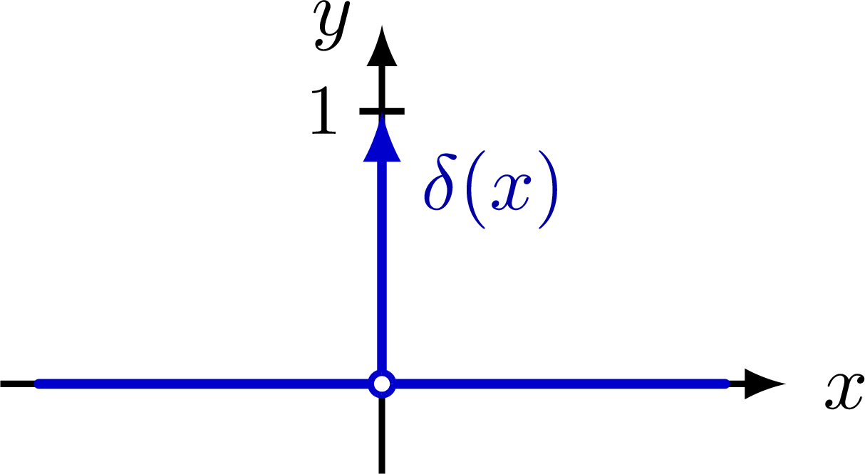
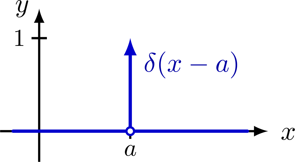
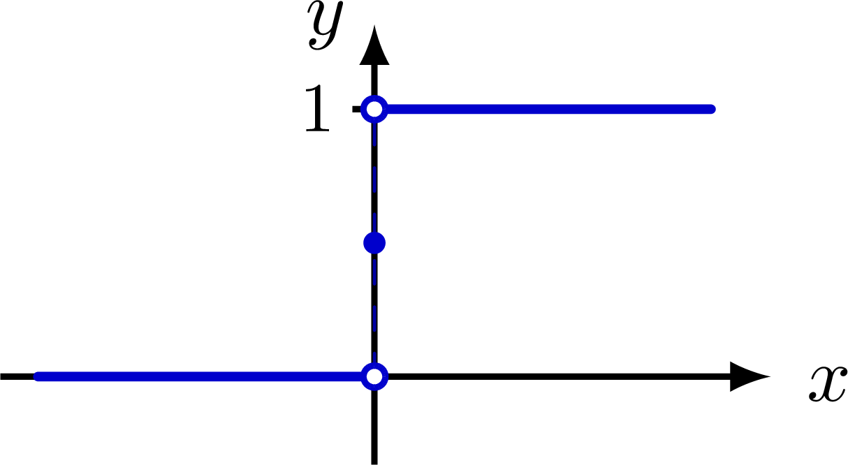
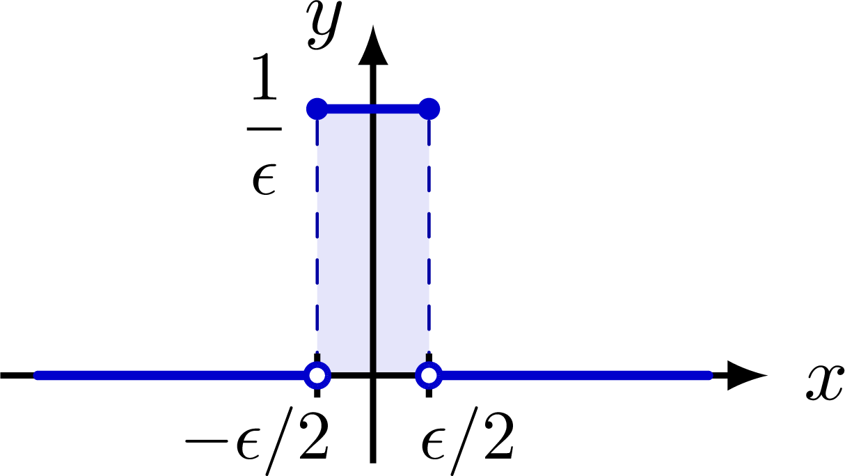
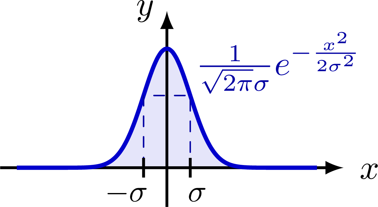
Delta function

Delta function indicated with an arrow, as well as different ways of defining the delta function as a limit of a distribution with fixed integral of 1.
For more Fourier analysis figures, please see the “fourier analysis” tag. These figures are used in Ben Kilminster’s lecture notes for PHY111.

Edit and compile if you like:

% Author: Izaak Neutelings (February 2021)
\documentclass[border=3pt,tikz]{standalone}
\usepackage{tikz}
\usepackage{physics}
\usepackage{xcolor}

\tikzset{>=latex} % for LaTeX arrow head
\colorlet{myred}{red!85!black}
\colorlet{myblue}{blue!80!black}
\colorlet{mydarkred}{myred!80!black}
\colorlet{mydarkblue}{myblue!80!black}
\tikzstyle{xline}=[myblue,very thick]
\def\tick#1#2{\draw[thick] (#1) ++ (#2:0.1) --++ (#2-180:0.2)}
\def\N{80}

\begin{document}


% DELTA FUNCTION
\def\xmin{-0.7*\T} % min x axis
\def\xmax{1.7}     % max x axis
\def\ymin{-0.4}    % min y axis
\def\ymax{1.6}     % max y axis
\def\A{0.76*\ymax} % amplitude
\begin{tikzpicture}
  \message{^^JDelta function}
  \def\a{0.4*\xmax}
  \tick{0,\A}{0} node[left=-1,scale=0.9] {1};
  \draw[->,thick] (0,\ymin) -- (0,\ymax) node[left] {$y$};
  \draw[->,thick] (-\xmax,0) -- (\xmax+0.1,0) node[below=1,right=1] {$x$};
  \draw[xline,line cap=round] (-0.9*\xmax,0) -- (0.9*\xmax,0);
  \draw[xline,->] (0,0) --++ (0,\A) node[mydarkblue,below right=1] {$\delta(x)$};
  \draw[xline,thick,fill=white] (0,0) circle(0.05);
\end{tikzpicture}


% DELTA FUNCTION - shift
\begin{tikzpicture}
  \message{^^JDelta function - shift}
  \def\a{0.70*\xmax}
  \tick{-\a,\A}{0} node[left=-1,scale=0.9] {1};
  \tick{0,0}{90} node[below=-1,scale=0.9] {$a$};
  \draw[->,thick] (-\a,\ymin) -- (-\a,\ymax) node[left] {$y$};
  \draw[->,thick] (-\xmax,0) -- (\xmax+0.1,0) node[below=1,right=1] {$x$};
  \draw[xline,line cap=round] (-0.9*\xmax,0) -- (0.9*\xmax,0);
  \draw[xline,->] (0,0) -- (0,\A) node[mydarkblue,below right=1] {$\delta(x-a)$};
  \draw[xline,thick,fill=white] (0,0) circle(0.05);
\end{tikzpicture}


% STEP FUNCTION
\begin{tikzpicture}
  \message{^^JStep function}
  \def\A{0.76*\ymax} % amplitude
  \draw[->,thick] (0,\ymin) -- (0,\ymax) node[left] {$y$};
  \draw[->,thick] (-\xmax,0) -- (\xmax+0.1,0) node[below=1,right=1] {$x$};
  \tick{0,\A}{0} node[left=-1,scale=0.9] {1};
  \draw[xline,very thick,line cap=round]
    (-0.9*\xmax,0) -- (0,0)
    (0,\A) -- (0.9*\xmax,\A);
  \draw[mydarkblue,dashed,thin,line cap=round]
    (0,0) -- (0,\A);
  \fill[xline] (0,\A/2) circle(0.05);
  \draw[xline,thick,fill=white] (0,0) circle(0.05);
  \draw[xline,thick,fill=white] (0,\A) circle(0.05);
\end{tikzpicture}


% DELTA FUNCTION - RECTANGULAR FUNCTION
\begin{tikzpicture}
  \message{^^JDelta function - rectangular limit}
  \def\A{0.76*\ymax} % amplitude
  \def\T{0.15*\xmax} % width
  \fill[myblue!10] (-\T,0) rectangle (\T,\A);
  \draw[->,thick] (0,\ymin) -- (0,\ymax) node[left] {$y$};
  \draw[->,thick] (-\xmax,0) -- (\xmax+0.1,0) node[below=1,right=1] {$x$};
  \draw[xline,very thick,line cap=round]
    ( \T,\A) -- (-\T,\A) node[black,below=2,left=0,scale=0.9] {$\dfrac{1}{\epsilon}$}
    (-\T,0) -- ({-0.9*\xmax},0)
    ( \T,0) -- ({ 0.9*\xmax},0);
  \draw[mydarkblue,dashed,thin,line cap=round]
    (-\T,0) --++ (0,{\A})
    ( \T,0) --++ (0,{\A});
  \tick{-\T,0}{90} node[left=8,below=-3,scale=0.9] {\strut$-\epsilon/2$};
  \tick{ \T,0}{90} node[right=5,below=-3,scale=0.9] {\strut$\epsilon/2$};
  \fill[xline] (-\T,\A) circle(0.05);
  \fill[xline] ( \T,\A) circle(0.05);
  \draw[xline,thick,fill=white] (-\T,0) circle(0.05);
  \draw[xline,thick,fill=white] ( \T,0) circle(0.05);
\end{tikzpicture}


% DELTA FUNCTION - GAUSSIAN FUNCTION
\begin{tikzpicture}
  \message{^^JDelta function - Gaussian limit}
  \def\A{0.76*\ymax} % amplitude
  \def\T{0.14*\xmax} % width
  \fill[myblue!10,samples=\N,variable=\x,domain=-0.9*\xmax:0.9*\xmax]
    plot(\x,{\A*exp(-(\x/(\T))^2/2)});
  \draw[->,thick] (0,\ymin) -- (0,\ymax) node[left] {$y$};
  \draw[->,thick] (-\xmax,0) -- (\xmax+0.1,0) node[below=1,right=1] {$x$};
  \draw[xline,very thick,smooth,samples=\N,variable=\x,domain=-0.9*\xmax:0.9*\xmax]
    plot(\x,{\A*exp(-(\x/(\T))^2/2)});
  \node[mydarkblue,right=0] at (0.1*\xmax,0.67*\ymax)
    {$\frac{1}{\sqrt{2\pi}\sigma}e^{-\frac{x^2}{2\sigma^2}}$};
  \draw[mydarkblue,dashed,thin,line cap=round]
    (-\T,0) |- (\T,{\A*exp(-1/2)}) -- (\T,0);
  \tick{-\T,0}{90} node[left=5,below=-4,scale=0.9] {\strut$-\sigma$};
  \tick{ \T,0}{90} node[right=2,below=-4,scale=0.9] {\strut$\sigma$};
\end{tikzpicture}


\end{document}