Averaging functions

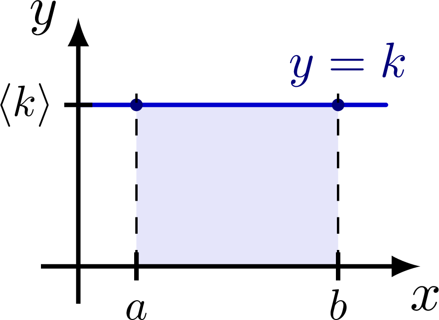
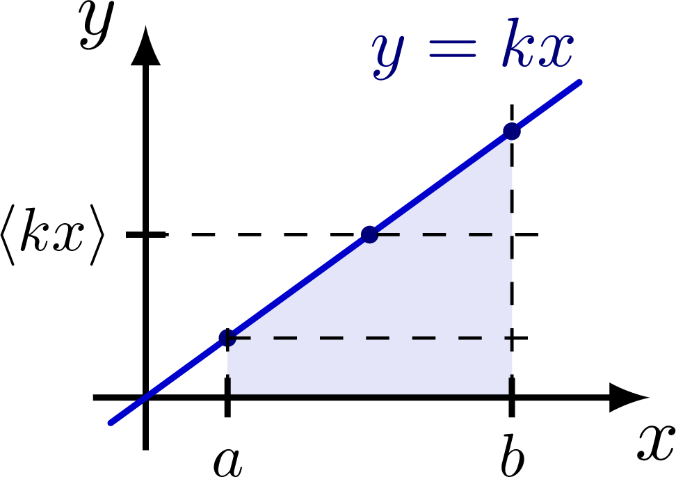
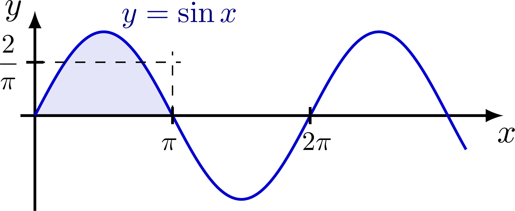
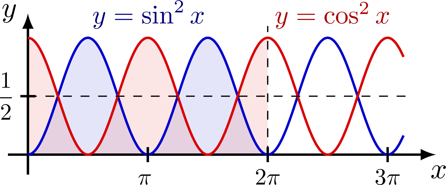
Some examples of averaging function via integration: a constant, linear, sine, sine squared and cosine squared function.

The average of the sine and cosine squared are needed to derive Fourier series, please see the “fourier analysis” tag for more related figures. These figures are used in Ben Kilminster’s lecture notes for PHY111.

Edit and compile if you like:

% Author: Izaak Neutelings (January 2021)
% http://pgfplots.net/tikz/examples/fourier-transform/
% https://tex.stackexchange.com/questions/127375/replicate-the-fourier-transform-time-frequency-domains-correspondence-illustrati
% https://www.dspguide.com/ch13/4.htm
\documentclass[border=3pt,tikz]{standalone}
\usepackage{amsmath}
\usepackage{tikz}
\usepackage{physics}
\usepackage{xcolor}
\usepackage[outline]{contour} % glow around text
\contourlength{1.0pt}

\tikzset{>=latex} % for LaTeX arrow head
\colorlet{myred}{red!85!black}
\colorlet{myblue}{blue!80!black}
\colorlet{mydarkred}{myred!80!black}
\colorlet{mydarkblue}{myblue!60!black}
\tikzstyle{xline}=[myblue,thick]
\def\tick#1#2{\draw[thick] (#1) ++ (#2:0.09) --++ (#2-180:0.18)}
\tikzstyle{myarr}=[myblue!50,-{Latex[length=3,width=2]}]
\def\N{100}

\begin{document}


% CONSTANT
\def\xmax{2.2} % max x axis
\def\ymax{1.6} % max y axis
\begin{tikzpicture}
  \message{^^JConstant}
  \def\a{0.17*\xmax} % first limit
  \def\b{0.76*\xmax} % last limit
  \def\k{0.65*\ymax} % constant value
  \fill[myblue!10] (\a,0) rectangle (\b,\k);
  \draw[->,thick] (0,-0.15*\ymax) -- (0,\ymax) node[left] {$y$};
  \draw[->,thick] (-0.15*\ymax,0) -- (\xmax,0) node[right=1,below] {$x$};
  \draw[xline,line cap=round] (0,\k) -- (0.9*\xmax,\k)
    node[mydarkblue,left=7,above=0,scale=0.9] {$y=k$};
  \fill[mydarkblue] (\a,\k) circle(0.04) (\b,\k) circle(0.04);
  \draw[dashed] (\a,0) --++ (0,1.07*\k);
  \draw[dashed] (\b,0) --++ (0,1.07*\k);
  \tick{\a,0}{90} node[below=-2.5,scale=0.8] {\strut$a$};
  \tick{\b,0}{90} node[below=-2.5,scale=0.8] {\strut$b$};
  \tick{0,\k}{0} node[left=-1,scale=0.8] {$\expval{k}$};
\end{tikzpicture}


% LINEAR
\begin{tikzpicture}
  \message{^^JLinear}
  \def\a{0.17*\xmax}  % first limit
  \def\b{0.76*\xmax}  % last limit
  \def\k{\ymax/\xmax} % slope coefficient
  \fill[myblue!10] (\a,0) -- (\a,\k*\a) -- (\b,\k*\b) |- cycle;
  \draw[->,thick] (0,-0.15*\ymax) -- (0,\ymax+0.1) node[left] {$y$};
  \draw[->,thick] (-0.15*\ymax,0) -- (\xmax+0.1,0) node[right=1,below] {$x$};
  \draw[xline,line cap=round]
    (-0.1*\ymax,-0.1*\k*\ymax) -- (0.9*\xmax,0.9*\k*\xmax)
    node[mydarkblue,above left=-3,scale=0.9] {$y=kx$};
  \fill[mydarkblue]
    (\a,\k*\a) circle(0.04) (\b,\k*\b) circle(0.04)
    ({(\b+\a)/2},{\k*(\b+\a)/2}) circle(0.04);
  \draw[dashed] (\a,0) --++ (0,1.25*\k*\a);
  \draw[dashed] (\b,0) --++ (0,1.10*\k*\b);
  \draw[dashed] (0,{\k*(\b+\a)/2}) --++ (1.1*\b,0);
  \draw[dashed] (\a,\k*\a) --++ ({1.1*(\b-\a)},0);
  \tick{\a,0}{90} node[below=-2,scale=0.8] {\strut$a$};
  \tick{\b,0}{90} node[below=-2,scale=0.8] {\strut$b$};
  \tick{0,{\k*(\b+\a)/2}}{0} node[left=-1,scale=0.8] {$\expval{kx}$};
\end{tikzpicture}


% SINE
\def\xmax{4.8} % max x axis
\begin{tikzpicture}
  \message{^^JSine}
  \def\ymax{1.0} % max y axis
  \def\T{0.60*\xmax} % period
  \def\A{0.88*\ymax} % amplitude
  \fill[myblue!10,samples=\N,smooth,variable=\x,domain=0:\T/2]
    plot(\x,{\A*sin(360/(\T)*\x)});
  \draw[->,thick] (0,-\ymax) -- (0,\ymax+0.1) node[left] {$y$};
  \draw[->,thick] (-0.15*\ymax,0) -- (\xmax+0.1,0) node[right=1,below] {$x$};
  \draw[xline,samples=\N,smooth,variable=\x,domain=0:0.94*\xmax]
    plot(\x,{\A*sin(360/(\T)*\x)});
  \draw[dashed] (0,2*\A/pi) --++ (0.53*\T,0);
  \draw[dashed] (0.5*\T,0) --++ (0,2.4*\A/pi);
  \tick{\T/2,0}{90} node[left=1,below=-2,scale=0.8] {\strut$\pi$}; %{\strut\contour{white}{$\pi$}};
  \tick{\T,0}{90} node[right=2,below=-2,scale=0.8] {\strut$2\pi$}; %{\strut\contour{white}{$2\pi$}};
  \tick{0,2*\A/pi}{0} node[left=-1,scale=0.8] {$\dfrac{2}{\pi}$};
  \node[above right=-2,mydarkblue,scale=0.9] at (0.3*\T,\A) {$y=\sin x$};
\end{tikzpicture}


% SINE^2
\begin{tikzpicture}
  \message{^^JSine}
  \def\T{0.60*\xmax} % period
  \def\A{0.88*\ymax} % amplitude
  \fill[myblue!10,samples=\N,smooth,variable=\x,domain=0:\T]
    plot(\x,{\A*sin(360/(\T)*\x)^2});
  \fill[myred!50,opacity=0.2,samples=\N,smooth,variable=\x,domain=0:\T]
    (0,0) -- plot(\x,{\A*cos(360/(\T)*\x)^2}) |- cycle;
  \draw[->,thick] (0,-0.15*\ymax) -- (0,\ymax+0.1) node[left] {$y$};
  \draw[->,thick] (-0.15*\ymax,0) -- (\xmax+0.1,0) node[right=1,below] {$x$};
  \draw[xline,samples=\N,smooth,variable=\x,domain=0:0.94*\xmax]
    plot(\x,{\A*sin(360/(\T)*\x)^2});
  \draw[xline,myred,samples=\N,smooth,variable=\x,domain=0:0.94*\xmax]
    plot(\x,{\A*cos(360/(\T)*\x)^2});
  \draw[dashed] (0,\A/2) --++ (0.96*\xmax,0); %1.05*\T
  \draw[dashed] (\T,0) --++ (0,1.1*\A);
  \tick{\T/2,0}{90} node[left=1,below=-2,scale=0.8] {\strut$\pi$};
  \tick{\T,0}{90} node[right=0,below=-2,scale=0.8] {\strut$2\pi$};
  \tick{1.5*\T,0}{90} node[right=0,below=-2,scale=0.8] {\strut$3\pi$};
  \tick{0,\A/2}{0} node[left=-1,scale=0.8] {$\dfrac{1}{2}$};
  \node[above right=0,mydarkblue,scale=0.9] at (0.23*\T,\A) {$y=\sin^2x$};
  \node[above right=0,mydarkred,scale=0.9] at (0.99*\T,\A) {$y=\cos^2x$};
\end{tikzpicture}


\end{document}