Magnetic field plots

Edit and compile if you like:

1
2
3
4
5
6
7
8
9
10
11
12
13
14
15
16
17
18
19
20
21
22
23
24
25
26
27
28
29
30
31
32
33
34
35
36
37
38
39
40
41
% Author: Izaak Neutelings (February 2020)
% page 8 https://archive.org/details/StaticAndDynamicElectricity
% https://tex.stackexchange.com/questions/56353/extract-x-y-coordinate-of-an-arbitrary-point-on-curve-in-tikz
% https://tex.stackexchange.com/questions/412899/tikz-calculate-and-store-the-euclidian-distance-between-two-coordinates
\documentclass[border=3pt,tikz]{standalone}
\usepackage{amsmath} % for \dfrac
\usepackage{physics}
\usepackage{tikz,pgfplots}
\usetikzlibrary{angles,quotes} % for pic (angle labels)
\usetikzlibrary{decorations.markings}
\tikzset{>=latex} % for LaTeX arrow head
\usepackage{xcolor}
\colorlet{Bcol}{violet!90}
\tikzstyle{BField}=[thick,Bcol]
\def\tick#1#2{\draw[thick] (#1) ++ (#2:0.03*\ymax) --++ (#2-180:0.06*\ymax)}
\begin{document}
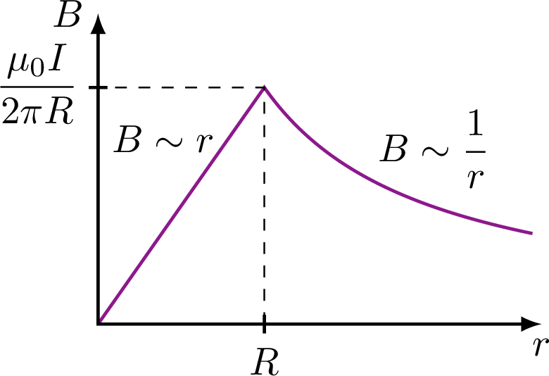
% MAGNETIC FIELD of a CHARGED SPHERE
\begin{tikzpicture}
  \def\xmax{4.4}
  \def\ymax{2.6}
  \def\kQ{2.85} % mu0 / 2*pi*R
  \def\R{1.4}
  \coordinate (O) at (0,0);
  \coordinate (X) at (\xmax,0);
  \coordinate (Y) at (0,\ymax);
  \coordinate (P) at (\R,\kQ/\R);
  \coordinate (Px) at (\R,0);
  \coordinate (Py) at (0,\kQ/\R);
  
  % PLOT
  \draw[BField,samples=100,smooth,variable=\x,domain=\R:0.96*\xmax]
    (O) -- (P) -- plot(\x,\kQ/\x);
  \node[above right] at (2.4,1.1) {$B \sim \dfrac{1}{r}$};
  \node[above left] at (0.82*\R,0.54*\ymax) {$B \sim r$};
  \draw[dashed]
 
 
הההההההההההההההההההההההההההההההההההההההההההההההההההההההההההההההההההההההההההההההההההההההההההההההההההההההההההההההההההההההההההההההההההההההההההההההההההההההההההההההההההההההההההההההההההההההההההההההההההההההההההההההההההההההההההההההההההההההההההההההההההההההההההההההה
XXXXXXXXXXXXXXXXXXXXXXXXXXXXXXXXXXXXXXXXXXXXXXXXXXXXXXXXXXXXXXXXXXXXXXXXXXXXXXXXXXXXXXXXXXXXXXXXXXXXXXXXXXXXXXXXXXXXXXXXXXXXXXXXXXXXXXXXXXXXXXXXXXXXXXXXXXXXXXXXXXXXXXXXXXXXXXXXXXXXXXXXXXXXXXXXXXXXXXXXXXXXXXXXXXXXXXXXXXXXXXXXXXXXXXXXXXXXXXXXXXXXXXXXXXXXXXXX