")


Edit and compile if you like:
% Author: Izaak Neutelings (March 2020)
\documentclass[border=3pt,tikz]{standalone}
\usepackage{amsmath} % for \dfrac
\usepackage{physics}
\usepackage{ifthen}
\usepackage{tikz,pgfplots}
\usepackage{tikz-3dplot}
\usepackage{auto-pst-pdf}
\usepackage{pst-magneticfield}
\usepackage[outline]{contour} % glow around text
\usetikzlibrary{angles,quotes} % for pic (angle labels)
\usetikzlibrary{arrows,arrows.meta}
\usetikzlibrary{calc}
\usetikzlibrary{decorations.markings}
\tikzset{>=latex} % for LaTeX arrow head
\usepackage{xcolor}
\colorlet{Ecol}{orange!90!black}
\colorlet{EcolFL}{orange!80!black}
\colorlet{veccol}{green!45!black}
\colorlet{projcol}{blue!70!black}
\colorlet{EFcol}{red!60!black}
\colorlet{Bcol}{violet!90}
\colorlet{Bcol1}{violet!80!blue!90}
\colorlet{Bcol2}{violet!80!red!90}
\colorlet{BFcol}{red!70!black}
\colorlet{veccol}{green!45!black}
\colorlet{Icol}{blue!70!black}
\colorlet{Ampcol}{green!60!black!70}
\tikzstyle{BField}=[->,thick,Bcol]
\tikzstyle{current}=[->,Icol,thick]
\tikzstyle{force}=[->,thick,BFcol]
\tikzstyle{vector}=[->,thick,veccol]
\tikzstyle{velocity}=[->,very thick,vcol]
\tikzstyle{metal}=[top color=black!15,bottom color=black!25,middle color=black!20,shading angle=10]
\tikzstyle{darkmetal}=[top color=black!40,bottom color=black!70,middle color=black!30,shading angle=10]
\tikzstyle{lightmetal}=[thin,black!20,top color=black!3,bottom color=black!6,middle color=black!1,shading angle=10]
\tikzstyle{proj}=[projcol!80,line width=0.08] %very thin
\tikzstyle{area}=[draw=veccol,fill=veccol!80,fill opacity=0.6]
\tikzstyle{measline}=[{Latex[length=3]}-{Latex[length=3]}]
\tikzset{
BFieldLine/.style={thick,Bcol,decoration={markings,mark=at position #1 with {\arrow{latex}}},
postaction={decorate}},
BFieldLine/.default=0.5,
Ampcurve/.style={Ampcol,decoration={markings,mark=at position #1 with {\arrow{latex}}},
postaction={decorate}},
Ampcurve/.default=0.55,
pics/Bin/.style={
code={
\def\R{0.12}
\draw[pic actions,line width=0.6,#1,fill=white] % ,thick
(0,0) circle (\R) (-135:.75*\R) -- (45:.75*\R) (-45:.75*\R) -- (135:.75*\R);
}},
pics/Bout/.style={
code={
\def\R{0.12}
\draw[pic actions,line width=0.6,#1,fill=white] (0,0) circle (\R);
\fill[pic actions,#1] (0,0) circle (0.3*\R);
}},
pics/Bin/.default=Bcol,
pics/Bout/.default=Bcol,
}
\tikzstyle{measure}=[fill=white,midway,outer sep=2]
%\newcommand\arrmark[1]{mark=at position #1 with {\arrow{latex}}}
%\def\myarrmark#1{mark=at position #1 with {\arrow{latex}}}
\contourlength{1.4pt}
% RING SHADING
\makeatletter
\pgfdeclareradialshading[tikz@ball]{ring}{\pgfpoint{0cm}{0cm}}%
{rgb(0cm)=(1,1,1);
rgb(0.719cm)=(1,1,1);
color(0.72cm)=(tikz@ball);
rgb(0.9cm)=(1,1,1)}
\tikzoption{ring color}{\pgfutil@colorlet{tikz@ball}{#1}\def\tikz@shading{ring}\tikz@addmode{\tikz@mode@shadetrue}}
\makeatother
\begin{document}
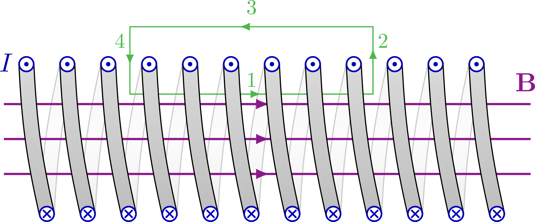
% SOLENOID MAGNETIC FIELD + Amp�re's law
\contourlength{1.0pt}
\begin{tikzpicture}
\message{Loop with Ampere's law start. ^^J}
\def\R{1}
\def\N{12}
\def\NB{3}
\def\L{6}
\def\t{0.20*\R}
\def\w{\L/(\N-1)}
%\draw[current] (-0.6*\R,-0.01*\R) arc (-94:-86:{0.6*\R/sin(4)})
% node[midway,below=0.6] {\contour{white}{$I$}};
% WIRE BACK
\foreach \i [evaluate={\x=-\L/2+(\i-1)*\w; \ang=atan(4*\R/(\w));}] in {1,...,\N}{
\ifthenelse{\i<\N}{
\draw[lightmetal]
({\x+\w/2},-\R)++(\ang+90:\t/2) to[out=\ang+5,in=\ang-185]++ (\ang:2.02*\R) -- ({\x+\w},\R)
--++ (\ang-90:\t/2) to[out=\ang-185,in=\ang+5]++ (\ang-180:2.02*\R) -- cycle;
}{}
}
% MAGNETIC FIELDLINES
\foreach \i [evaluate={\y=(\i-\NB/2-0.5)*1.4*\R/\NB}] in {1,...,\NB}{
\draw[BFieldLine={0.505}] (-0.55*\L,\y) -- (0.62*\L,\y);
}
\node[Bcol] at (0.61*\L,0.76*\R) {$\vb{B}$};
% AMPERE's LOOP
\draw[Ampcol]
(-0.27*\L,0.6*\R) -| (0.27*\L,1.5*\R) -| cycle;
\draw[Ampcurve={0.54}]
(-0.27*\L,0.6*\R) -- (0.27*\L,0.6*\R) node[midway,above,scale=0.8] {1};
\draw[Ampcurve={0.68}]
( 0.27*\L,0.6*\R) -- (0.27*\L,1.5*\R) node[midway,above=3,above right=-1,scale=0.8] {2};
\draw[Ampcurve={0.55}]
( 0.27*\L,1.5*\R) -- (-0.27*\L,1.5*\R) node[midway,above=3,above=-1,scale=0.8] {3};
\draw[Ampcurve={0.57}]
(-0.27*\L,1.5*\R) -- (-0.27*\L,0.6*\R) node[midway,above=3,above left=-1,scale=0.8] {4};
% WIRE FRONT
\foreach \i [evaluate={\x=-\L/2+(\i-1)*\w; \ang=atan(4*\R/(\w));}] in {1,...,\N}{
\draw[metal] (\x,\R)++(-90-\ang:\t/2) --++ (90-\ang:\t) to[out=-\ang-5,in=185-\ang]++ (-\ang:2.02*\R)
-- ({\x+\w/2},-\R) --++ (-90-\ang:\t/2) to[out=185-\ang,in=-\ang-5] cycle;
\pic[scale=0.81] at ({\x+\w/2},-\R) {Bin={Icol}};
\pic[scale=0.81] at (\x,\R) {Bout={Icol}};
}
\node[Icol] at (-0.545*\L,1.02*\R) {$I$};
% \foreach \i [evaluate={\x=-\L/2+(\i-1)*\L/(\N-1); \ang=atan(2*\R*(\N-1)/\L)}] in {1,...,\N}{
% \ifthenelse{\i<\N}{
% \draw[lightmetal]
% (\x,-\R)++(\ang+90:\t/2) --++ (\ang:2.08*\R) -- ({\x+\L/(\N-1)},\R) --++(\ang-90:\t/2) --++ (\ang-180:2.08*\R) ;
% }{}
% \draw[metal] (\x-\t/2,\R) arc (180:0:\t/2) --++ (0,-2*\R) arc (0:-180:\t/2) -- cycle;
% \pic[scale=0.81] at (\x,-\R) {Bin={Icol}};
% \pic[scale=0.81] at (\x,\R) {Bout={Icol}};
% }
\message{Loop with Ampere's law done. ^^J}
\end{tikzpicture}
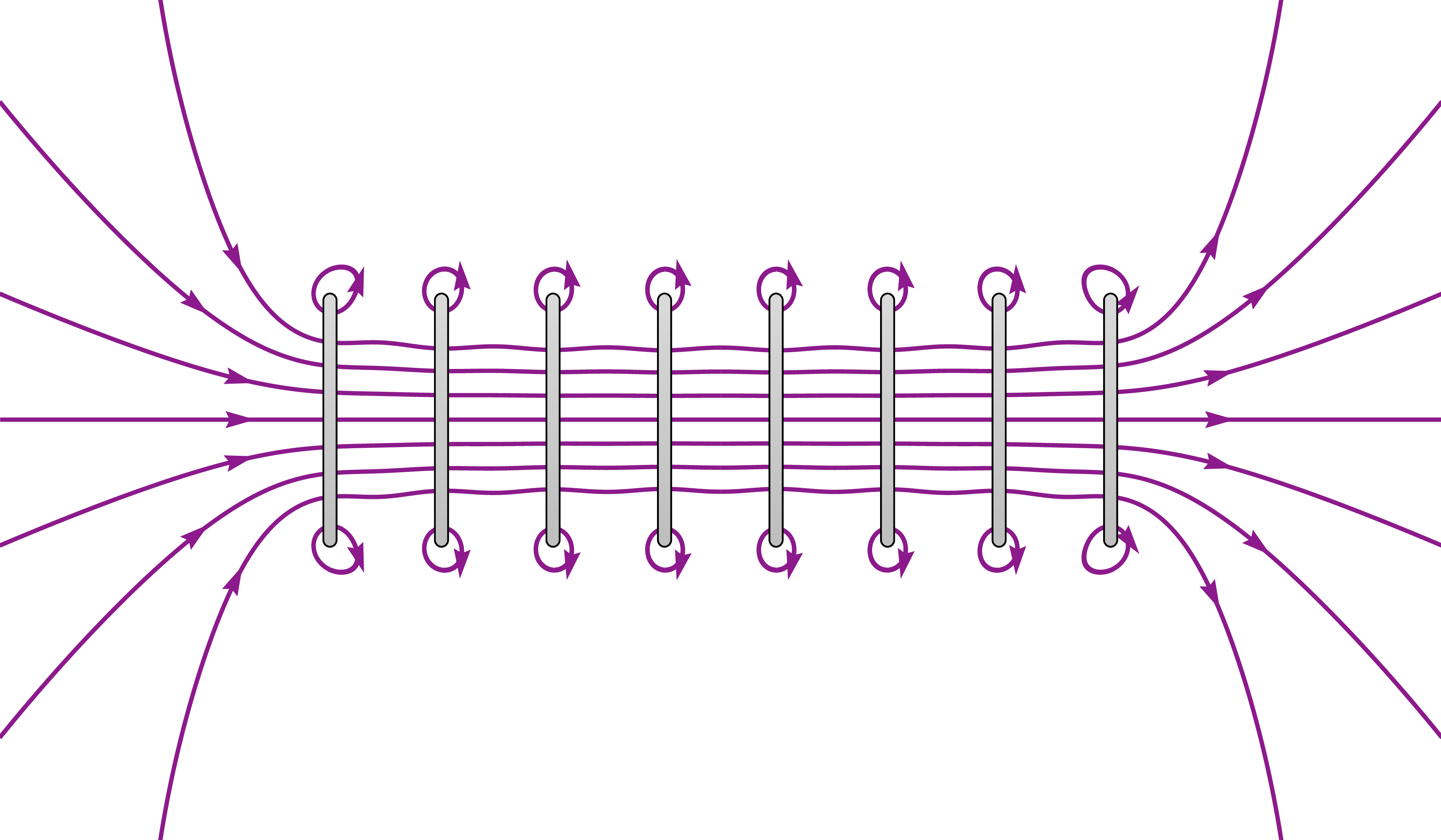
% SOLENOID MAGNETIC FIELD
\def\xmax{6}
\def\ymax{3.5}
\begin{tikzpicture}[shift={(\xmax+0.024,\ymax+0.024)}]
\message{Solenoid start. ^^J}
\def\R{1}
\def\N{8}
\def\L{6.5}
\def\t{0.11*\R}
\begin{scope} %[shift={(3,3)}]
\clip (-\xmax,-\ymax) rectangle (\xmax,\ymax);
\begin{pspicture*}(-\xmax,-\ymax)(\xmax,\ymax) %dotangle=-90
\rotatebox{-90}{
\psframe[linecolor=white](-\ymax,-\xmax)(\ymax,\xmax)
\psmagneticfield[
N=\N,R=\R,L=\L,
nL=4,pointsB=1000,%PasB=0.002,
nS=1,numSpires=,PasS=0.001,pointsS=1200, %2 3 4 5 6 7,PasS=0.004
linewidth=1.0pt,linecolor=Bcol,drawSelf=false
](-\ymax,-\xmax)(\ymax,\xmax)}
\end{pspicture*}
\end{scope}
\foreach \i [evaluate={\x=-\L/2+(\i-1)*\L/(\N-1);}] in {1,...,\N}{
\draw[metal] (\x-\t/2,\R) arc (180:0:\t/2) --++ (0,-2*\R) arc (0:-180:\t/2) -- cycle;
}
\message{Solenoid done. ^^J}
\end{tikzpicture}
\end{document}
Click to download: magnetic_field_solenoid.tex • magnetic_field_solenoid.pdf
Open in Overleaf: magnetic_field_solenoid.tex


Hi, how are you?
I have been trying to compile this on my beamer presentation. While the first one works without a glitch, the field lines never show in my presentation.
Any idea on why that is?
Thank you!
Hi Wagner, hard to say without looking at the tex and log file… Sorry I cannot be more helpful.
[8] Solenoid start.
./magnetism_lesson.tex:513: Undefined control sequence.
\c@lor@to@ps ->\PSTricks
_Not_Configured_For_This_Format
l.513 \end{frame}
? ./magnetism_lesson.tex:513: Undefined control sequence.
\XC@usec@lor …\expandafter \c@lor@to@ps #1#2\@@
\else \expandafter \expand…
l.513 \end{frame}
The only thing that I get are the “wires” of the solenoid, for some reason, which I cannot figure out why.
Thank you so much for your help
Hi Wagner,
The solenoid wires show up because it is drawn with TikZ, while the magnetic field is draw with PSTricks, which is an entirely separate package. While PSTricks can generate magnetic field lines for a given setup quite nicely, it requires some care for compiling correctly, despite the
auto-pst-pdfpackage, that is supposed to make it easier. I also had some issue in the past.I am afraid that I am familiar with this particular error, and I am not an expert in PSTricks, however after googling the error, I did find this discussion, which might be helpful to you?
https://groups.google.com/g/pretext-dev/c/sOC4ZP4AGpU
You will probably have to play around with different ways of compiling it, for example by adding
--shell-escape, or usingxelatexas compiler. In the discussion linked above, it seemed to work with(Btw, this website cannot run the example with “–shell-escape” for security reasons.)
I would suggested looking around with Google, or consulting the manuals for PSTricks,
pst-magneticfield, orauto-pst-pdf:https://tug.org/PSTricks/main.cgi/
https://ctan.org/pkg/pst-magneticfield
https://ctan.org/pkg/auto-pst-pdf
Or, you can save yourself some headache, and try to compile the figure separately once and load it as an external PDF into your tex file with
\includegraphics. A pre-compiled PDF can be found at the bottom of the post. I often do it like this to avoid code duplication, reduce complexity, and speed up compilation for bigger projects.Hope that helps… Let me know if you find a solution to compile it, as it might be useful to others!
Cheers,
Izaak
First of all, thank you very much, Izaak, for sharing your LaTex code. The pictures look fantastic and are also super useful for anyone working on similar projects.
I was experiencing the same problem as Wagner. I managed to overcome the issue and recreate Izaak’s drawing by compiling the document on Overleaf using XeLaTex. I had to separate the TikZ part from the PSTricks part using distinct environments for each. Then I had to ensure proper alignment by placing both PSTricks and TikZ content inside a TikZ node.
Here is the minimal working example:
\documentclass{standalone}
\usepackage{pst-magneticfield}
\colorlet{Bcol}{violet!90}
\usepackage{tikz}
\tikzstyle{metal}=[top color=black!15,bottom color=black!25,middle color=black!20,shading angle=10]
\begin{document}
% SOLENOID MAGNETIC FIELD
\def\xmax{6}
\def\ymax{3.5}
\def\R{1}
\def\N{8}
\def\L{6.5}
\def\t{0.11*\R}
\begin{tikzpicture}
\node[anchor=center]{
\begin{pspicture*}(-\xmax,-\ymax)(\xmax,\ymax) %dotangle=-90
\rotatebox{-90}{
\psframe[linecolor=white](-\ymax,-\xmax)(\ymax,\xmax)
\psmagneticfield[
N=\N,R=\R,L=\L,
nL=4,pointsB=1000,%PasB=0.002,
nS=1,numSpires=,PasS=0.001,pointsS=1200, %2 3 4 5 6 7,PasS=0.004
linewidth=1.0pt,linecolor=Bcol,drawSelf=false
](-\ymax,-\xmax)(\ymax,\xmax)}
\end{pspicture*}
};
\foreach \i [evaluate={\x=-\L/2+(\i-1)*\L/(\N-1);}] in {1,…,\N}{
\draw[metal]
(\x-\t/2,\R) arc (180:0:\t/2) –++ (0,-2*\R) arc (0:-180:\t/2) — cycle;
}
\end{tikzpicture}
\end{document}
I really hope this will be useful to others.