Osculating Circle

Edit and compile if you like:

\documentclass{article}
\usepackage{tikz}
\usepackage{tikz-3dplot}
\usetikzlibrary{math}
\usepackage{ifthen}
\usepackage[active,tightpage]{preview}
\PreviewEnvironment{tikzpicture}
\setlength\PreviewBorder{1pt}
%
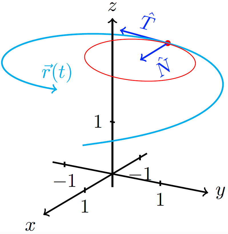
% File name: truncated-cylinder.tex
% Description: 
% A geometric representation of a truncated cylinder is shown.
% 
% Date of creation: September, 19th, 2021.
% Date of last modification: October, 9th, 2022.
% Author: Efraín Soto Apolinar.
% https://www.aprendematematicas.org.mx/author/efrain-soto-apolinar/instructing-courses/
% Source: page 48 of the 
% Glosario Ilustrado de Matem\'aticas Escolares.
% https://tinyurl.com/5udm2ufy
%
% Terms of use:
% According to TikZ.net
% https://creativecommons.org/licenses/by-nc-sa/4.0/
% Your commitment to the terms of use is greatly appreciated.
%
\begin{document}
%
\begin{center}
\tdplotsetmaincoords{70}{120}
%
\begin{tikzpicture}[tdplot_main_coords]
	% Components of the vector function
	\tikzmath{function equis(\t) {return cos((\t) r);};}
	\tikzmath{function ye(\t) {return sin((\t) r);};}
	\tikzmath{function zeta(\t) {return 0.5+0.25*sqrt(\t);};}
	% Components of the derivative f the vector function
	\tikzmath{function dequis(\t) {return -sin((\t) r);};}
	\tikzmath{function dye(\t) {return cos((\t) r);};}
	\tikzmath{function dzeta(\t) {return 0.125/sqrt(\t);};}
	% Components of the normal vector (second derivative of $\vec{r}(t)$
	\tikzmath{function ddequis(\t) {return -cos((\t) r);};}
	\tikzmath{function ddye(\t) {return -sin((\t) r);};}
	\tikzmath{function ddzeta(\t) {return -0.0625/(\t)^(1.5);};}
	% Evaluate everything at the point \tcero
	\pgfmathsetmacro{\tcero}{1.0*pi} 
	\pgfmathsetmacro{\ti}{0.25} % initial value for the plot
	\pgfmathsetmacro{\tf}{2.0*pi} % final value for the plot
	\pgfmathsetmacro{\n}{100}	% number of points
	\pgfmathsetmacro{\r}{2.0}	% auxiliary distance 
	\pgfmathsetmacro{\Px}{\r*equis(\tcero)}
	\pgfmathsetmacro{\Py}{\r*ye(\tcero)}
	\pgfmathsetmacro{\Pz}{\r*zeta(\tcero)}
	% Position of the node $\vec{r}(t)$
	\pgfmathsetmacro{\xf}{\r*equis(\tf)}
	\pgfmathsetmacro{\yf}{\r*ye(\tf)}
	\pgfmathsetmacro{\zf}{\r*zeta(\tf)}
	% Components of the tangent vector to $\vec{r}(t)$ at $t = \tcero$
	\pgfmathsetmacro{\drx}{dequis(\tcero)}
	\pgfmathsetmacro{\dry}{dye(\tcero)}
	\pgfmathsetmacro{\drz}{dzeta(\tcero)}
	% Components of the normal vector to $\vec{r}(t)$ at $t = \tcero$
	\pgfmathsetmacro{\ddrx}{ddequis(\tcero)}
	\pgfmathsetmacro{\ddry}{ddye(\tcero)}
	\pgfmathsetmacro{\ddrz}{ddzeta(\tcero)}
	% Components of the unit tangent vector $\hat{T}$
	\pgfmathsetmacro{\Tmag}{sqrt(\drx*\drx+\dry*\dry+\drz*\drz)}
	\pgfmathsetmacro{\Tx}{\drx/\Tmag}
	\pgfmathsetmacro{\Ty}{\dry/\Tmag}
	\pgfmathsetmacro{\Tz}{\drz/\Tmag}
	% Componentes of the unit normal vector $\hat{N}$
	\pgfmathsetmacro{\Nmag}{sqrt(\ddrx*\ddrx+\ddry*\ddry+\ddrz*\ddrz)}
	\pgfmathsetmacro{\Nx}{\ddrx/\Nmag}
	\pgfmathsetmacro{\Ny}{\ddry/\Nmag}
	\pgfmathsetmacro{\Nz}{\ddrz/\Nmag}
	% Compute the curvature
	%\pgfmathsetmacro{\k}{\Nmag/\Tmag} % Not needed
	% Radius of curvature
	\pgfmathsetmacro{\rk}{\Tmag/\Nmag}
	% Coordinates of the center of the osculating circle
	\pgfmathsetmacro{\Cx}{\Px+\rk*\Nx}
	\pgfmathsetmacro{\Cy}{\Py+\rk*\Ny}
	\pgfmathsetmacro{\Cz}{\Pz+\rk*\Nz}
	% Negative part of the coordinate axis
	\draw[thick,->] (-1.25,0,0) -- (\r+0.5,0,0) node[below left] {$x$}; % $x$ axis
	\foreach \x in {-1,1}
		\draw[thick] (\x,0,0.05) -- (\x,0,-0.05) node [below] {$\x$};
	\draw[thick,->] (0,-1.25,0) -- (0,\r,0) node[right] {$y$}; % $y$ axis
	\foreach \y in {-1,1}
		\draw[thick] (0,\y,0.05) -- (0,\y,-0.05) node [below] {$\y$};
	\draw[thick] (0,0,-0.25) -- (0,0,1.0); % $z$ axis (first part)
	% Point P
	\fill[red] (\Px,\Py,\Pz) circle (1.5pt);
	% Tangent vector $\hat{T}$
	\draw[blue,thick,->,shift={(\Px,\Py,\Pz)}] (0,0,0) -- (\Tx,\Ty,\Tz) node[midway,sloped,above] {$\hat{T}$};	
	% Normal vector $\hat{N}$
	\draw[blue,thick,->,shift={(\Px,\Py,\Pz)}] (0,0,0) -- (\Nx,\Ny,\Nz) node[midway,sloped,below] {$\hat{N}$};	
	% Graph of the vector function $\vec{r(t)}$
	\draw[cyan,thick,->] plot[domain=\ti:\tf,smooth,variable=\t,samples=\n] ({\r*equis(\t)},{\r*ye(\t)},{\r*zeta(\t)});
	\node[cyan,above,->] at (\xf,\yf,\zf) {$\vec{r}(t)$};
	% Last part of the $z$ axis
	\draw[thick,->] (0,0,1.0) -- (0,0,\r+1.0) node[above] {$z$}; % Eje z
	\foreach \z/\posicion in {1/left}
		\draw[thick] (0,0.05,\z) -- (0,-0.05,\z) node [\posicion] {$\z$};
	% The osculating circle
	\draw[red,shift={(\Cx,\Cy,\Cz)}] 
		plot[domain=0:2*pi,smooth,variable=\t,samples=100] ({\rk*cos(\t r)},{\rk*sin(\t r)},{-\rk*\drz*sin(\t r)});
\end{tikzpicture}
\end{center}
%
\end{document}