")


Some basic PV (pressure-volume) diagrams with isothermal, isochoric, isobaric or adiabatic processes, including the Otto cycle and Carnot cycle. For more figures related to thermodynamics, see the “thermodynamics” category.
PV diagram for a constant pressure P: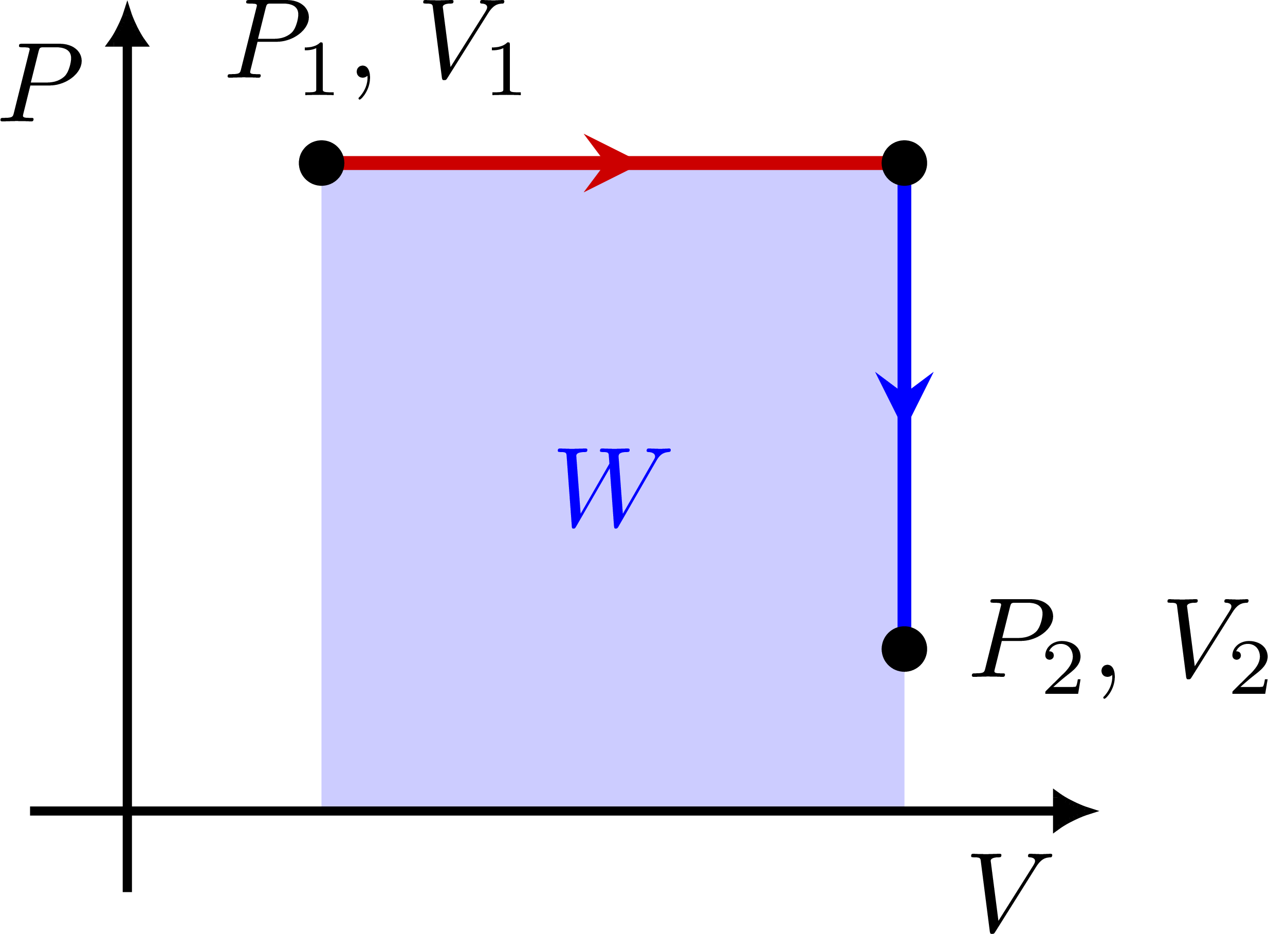
PV diagram for a constant volume V: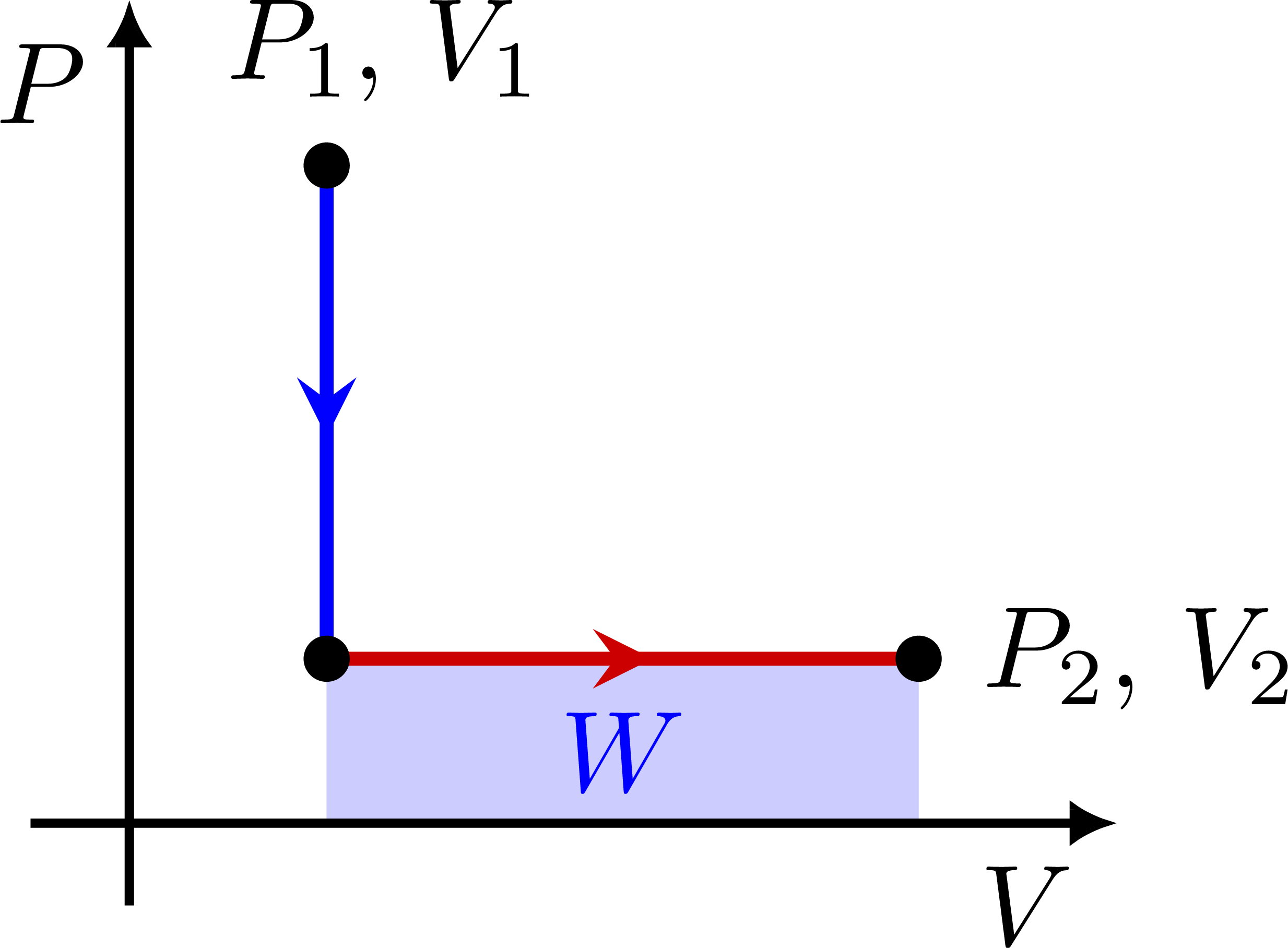
PV diagram with an isotherm (constant temperature T):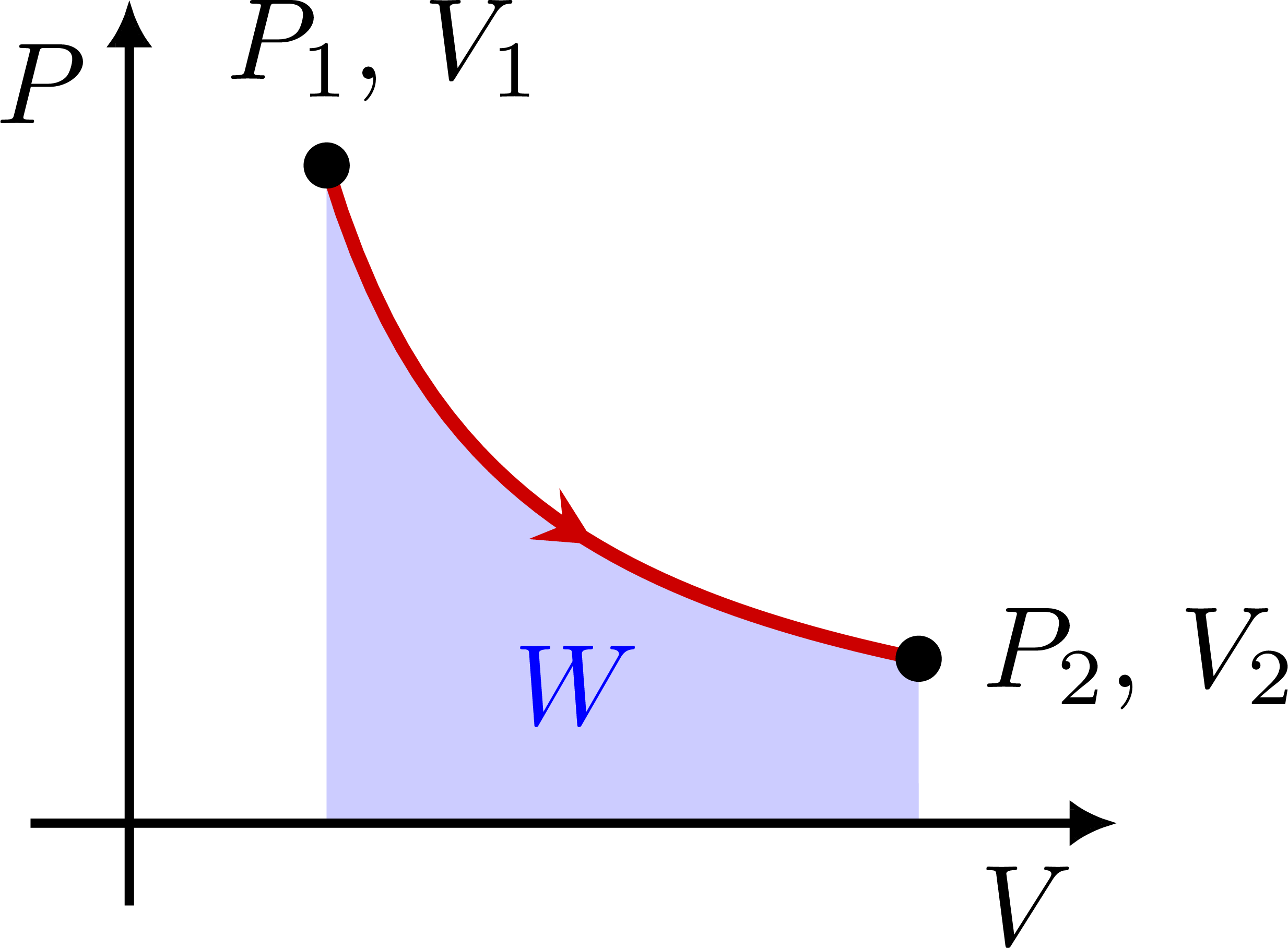
PV diagram of a simple, engine: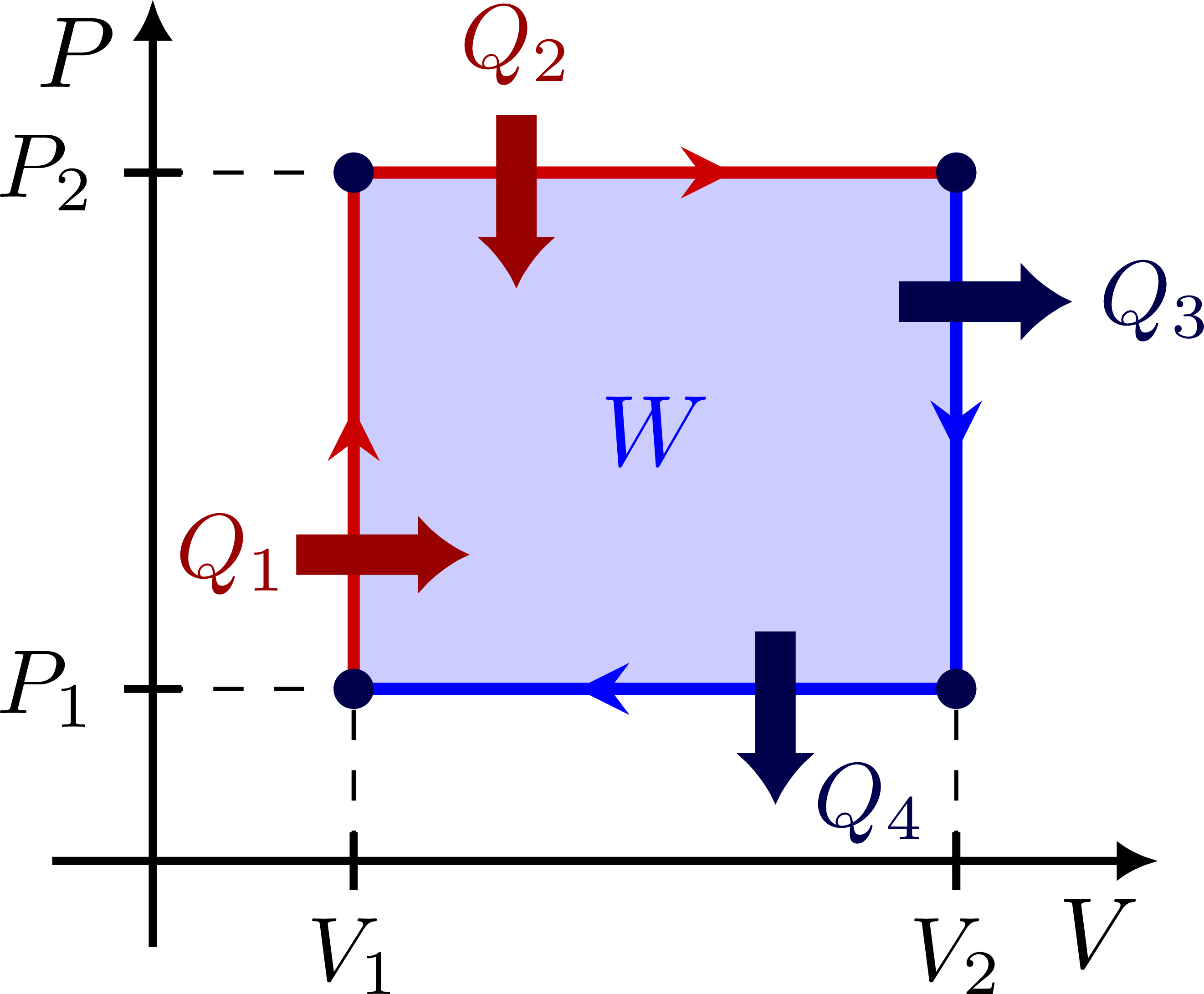
Connecting isotherms via different paths in PV by adding heat Q to the system: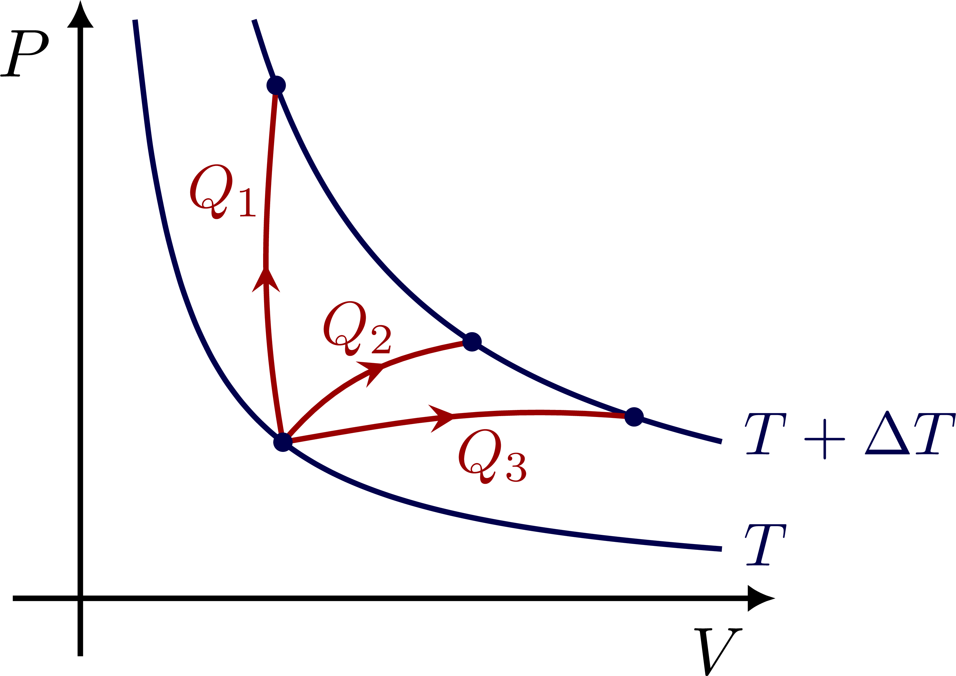
Specific heat capacities for constant pressure (CP) or constant volume (CV):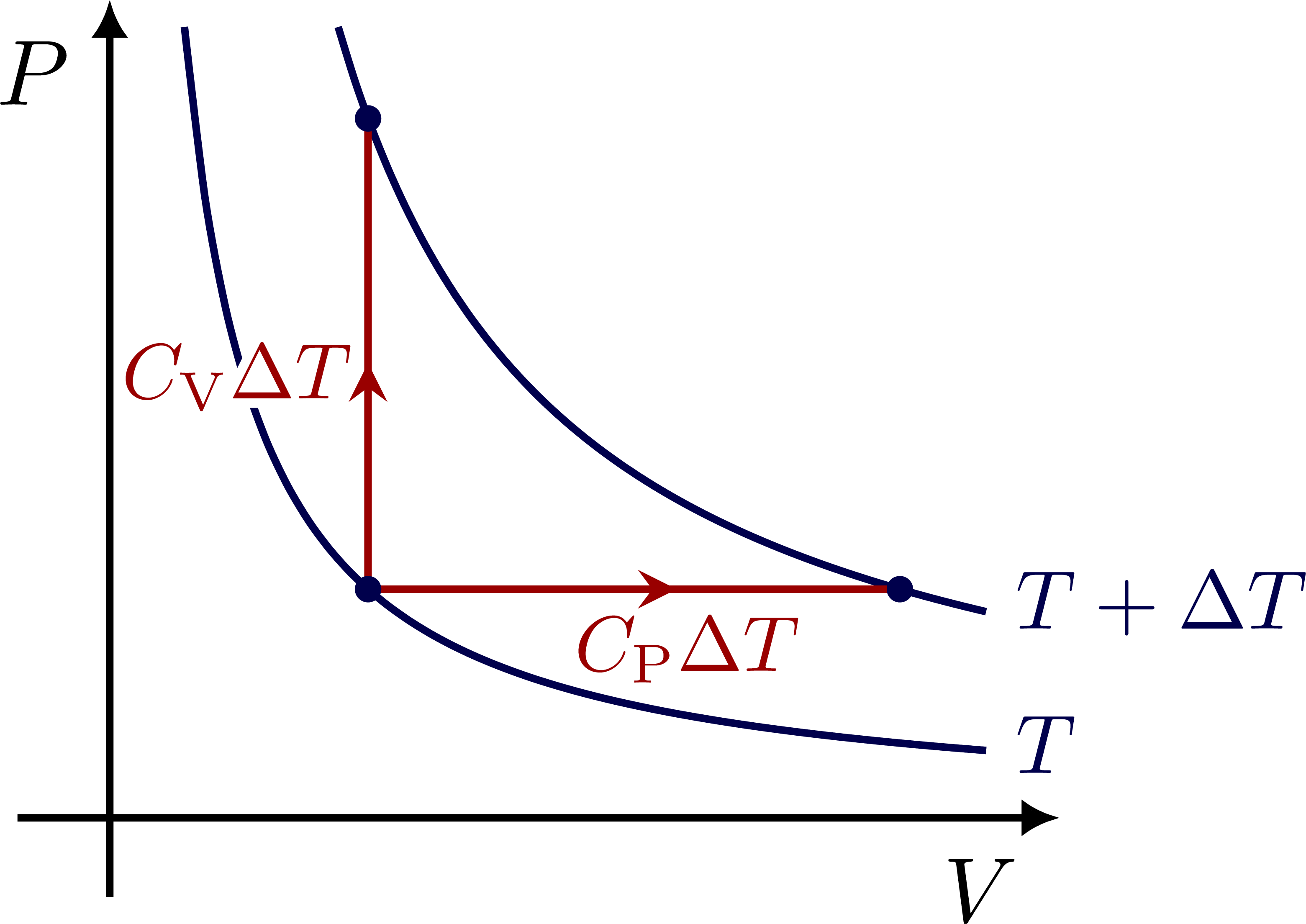
Connecting isotherms with an adiabatic process: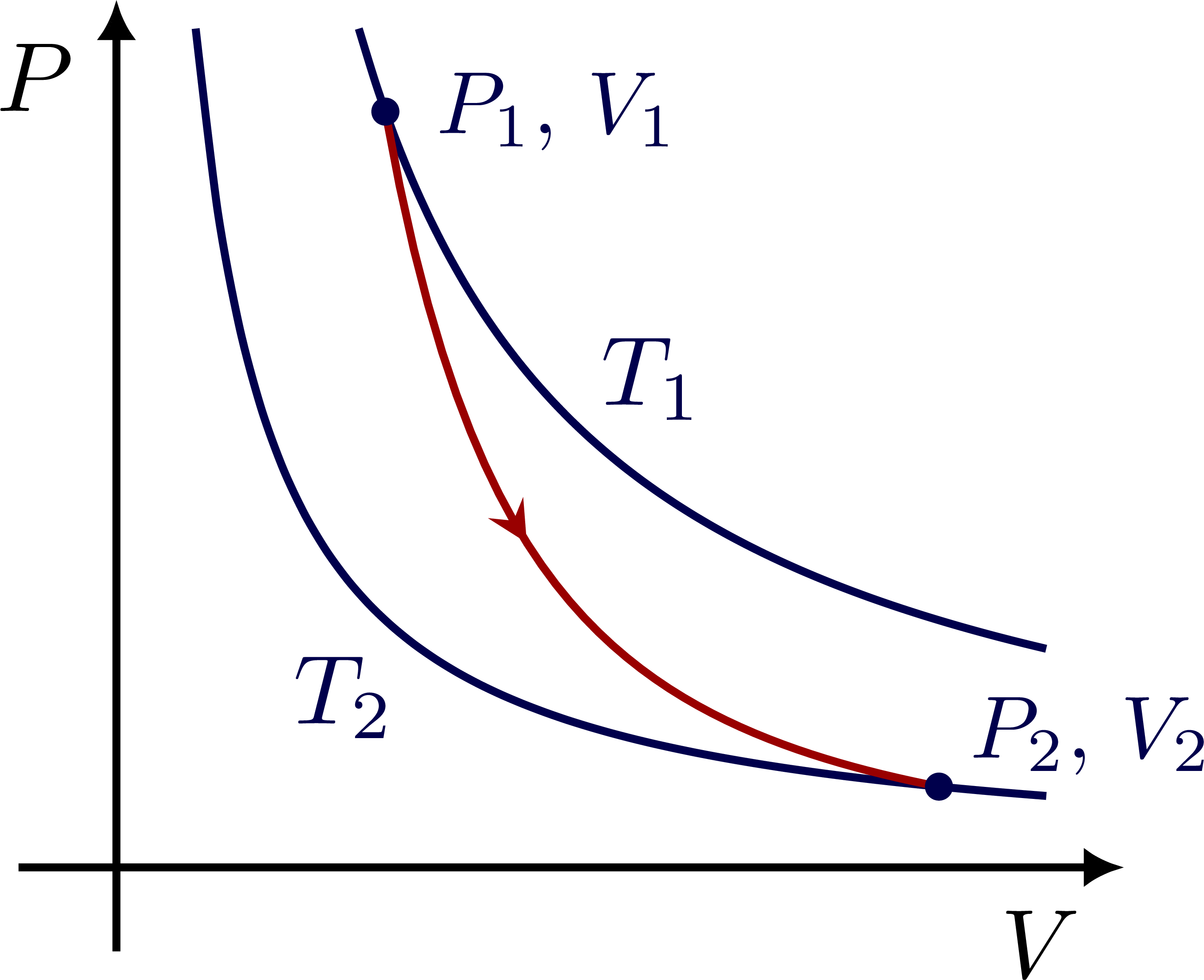
The work done by an adiabatic process is given by the area: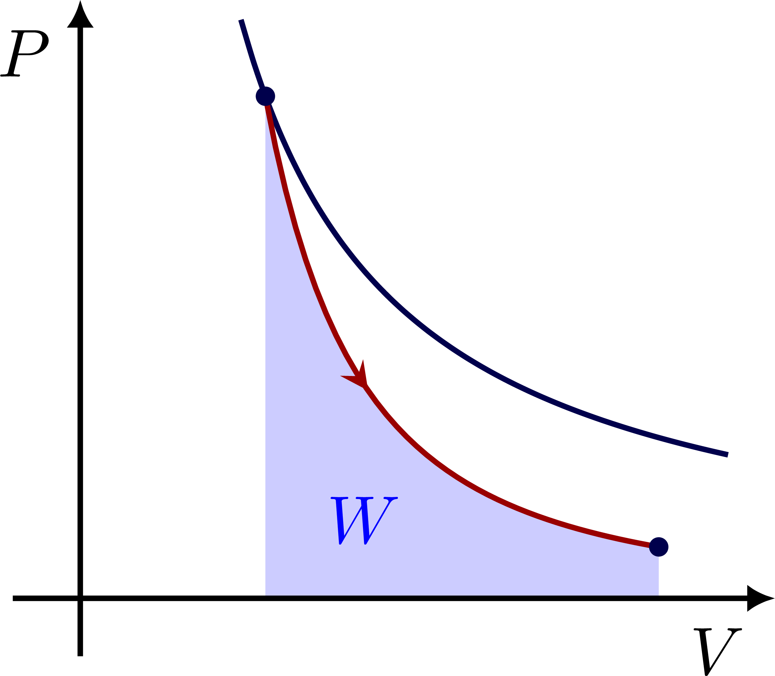
PV diagram for the Otto cycle: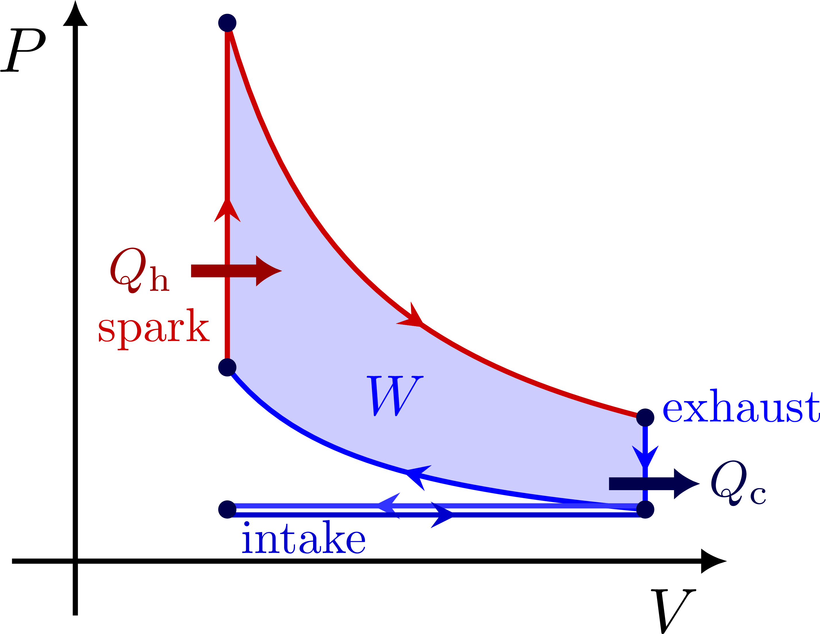
PV diagram for the Carnot cycle: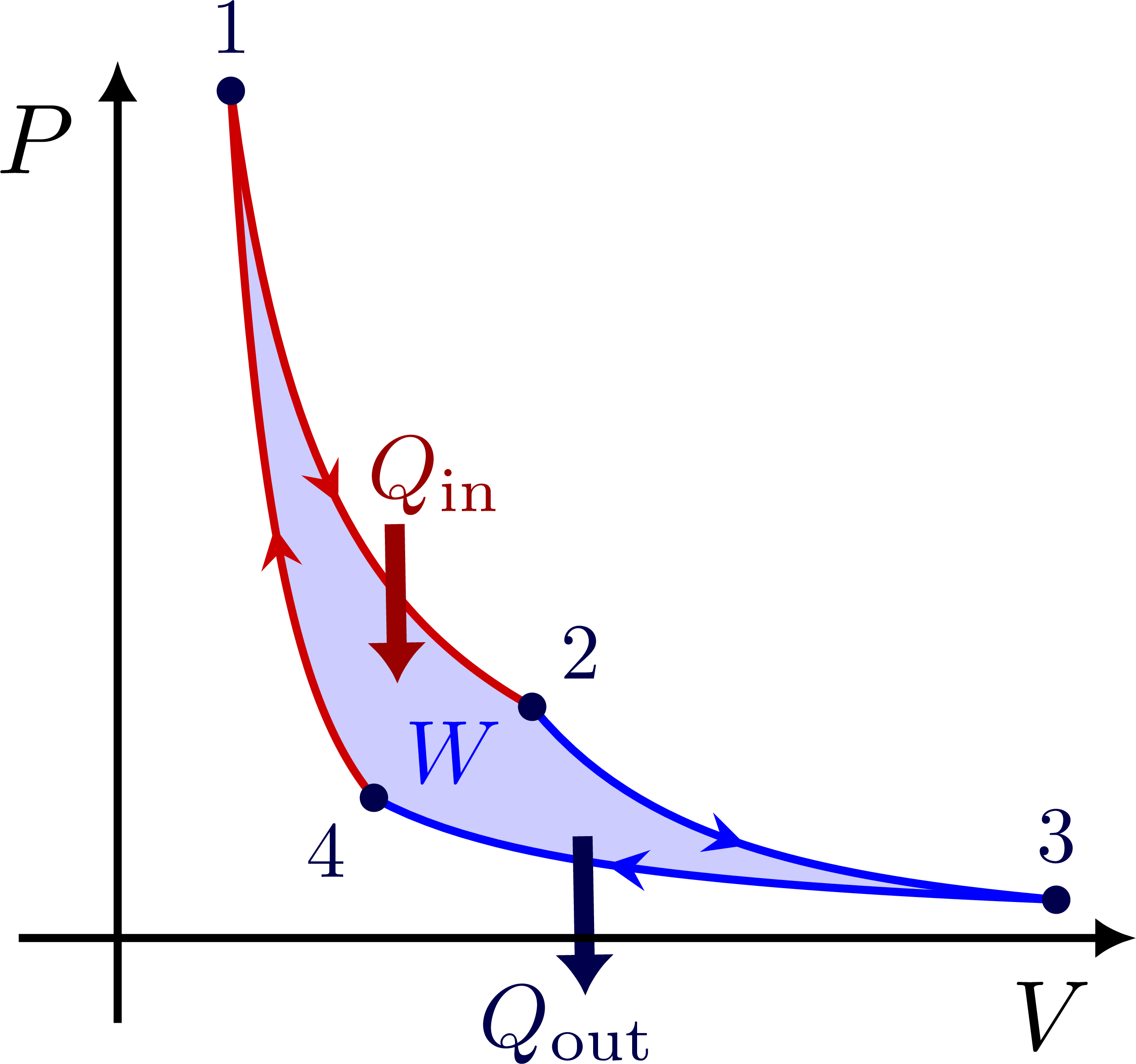
Edit and compile if you like:
% Author: Izaak Neutelings (June, 2018)
\documentclass[border=3pt,tikz]{standalone}
\usepackage{tikz}
\usepackage{amsmath} % for \text
\usepackage[outline]{contour} % glow around text
\usetikzlibrary{arrows.meta} % to control arrow size
\tikzset{>={Latex[length=4,width=4]}} % for LaTeX arrow head
\usetikzlibrary{calc,decorations.markings,arrows.meta}
\usepackage{xcolor} % for colored text
\contourlength{1.2pt}

\colorlet{mylightblue}{blue!20}
\colorlet{myblue}{blue!80!black}
\colorlet{mydarkblue}{blue!30!black}
\colorlet{mylightred}{red!10}
\colorlet{myred}{red!80!black}
\colorlet{mydarkred}{red!60!black}
\colorlet{mydarkgreen}{green!30!black}

%\tikzstyle{midarr}=[decoration={markings,mark=at position 0.5 with {\arrow{stealth}}},postaction={decorate}]
\tikzset{
  midarr/.style={decoration={markings,mark=at position #1 with {\arrow{stealth}}},postaction={decorate}},
  midarr/.default=0.5
}

\def\xtick#1#2{\draw[thick] (#1)++(0,.1) --++ (0,-.2) node[below=-.5pt,scale=0.9] {#2};}
\def\ytick#1#2{\draw[thick] (#1)++(.1,0) --++ (-.2,0) node[left=-.5pt,scale=0.9] {#2};}

\begin{document}


% PV diagram - constant P
\def\N{40} % number of plot samples
\def\xmax{3}
\def\ymax{2.5}
\begin{tikzpicture}

  % AREA
  \coordinate (A) at (.2*\xmax,.8*\ymax);
  \coordinate (B) at (.8*\xmax,.8*\ymax);
  \coordinate (C) at (.8*\xmax,.2*\ymax);
  \fill[mylightblue] (A) rectangle (C|-0,0) node[midway,blue] {$W$};

  % LINE
  \draw[very thick,midarr=.55,myred] (A) -- (B);
  \draw[very thick,midarr=.55,blue] (B) -- (C);
  \fill (A) circle(0.07) node[right=5,above=2] {$P_1$, $V_1$};
  \fill (B) circle(0.07);
  \fill (C) circle(0.07) node[right=2] {$P_2$, $V_2$};

  % AXIS
  \draw[->,thick] (0,-0.1*\ymax) -- (0,\ymax) node[anchor=north east] {$P$};
  \draw[->,thick] (-0.1*\xmax,0) -- (\xmax,0) node[anchor=north east] {$V$};

\end{tikzpicture}


% PV diagram - constant V
\begin{tikzpicture}

  % AREA
  \coordinate (A) at (.2*\xmax,.8*\ymax);
  \coordinate (B) at (.2*\xmax,.2*\ymax);
  \coordinate (C) at (.8*\xmax,.2*\ymax);
  \fill[mylightblue] (B) rectangle (C|-0,0) node[below=-6,midway,blue] {$W$};

  % LINE
  \draw[very thick,midarr=.55,blue] (A) -- (B);
  \draw[very thick,midarr=.55,myred] (B) -- (C);
  \fill (A) circle(0.07) node[right=5,above=2] {$P_1$, $V_1$};
  \fill (B) circle(0.07);
  \fill (C) circle(0.07) node[right=2] {$P_2$, $V_2$};

  % AXIS
  \draw[->,thick] (0,-0.1*\ymax) -- (0,\ymax) node[anchor=north east] {$P$};
  \draw[->,thick] (-0.1*\xmax,0) -- (\xmax,0) node[anchor=north east] {$V$};

\end{tikzpicture}


% PV diagram - isotherm
\begin{tikzpicture}
  \def\isotherm{(A) to[out=-60,in=170] (B)}
  \def\T{1.2}
  \def\xa{.2*\xmax}
  \def\xb{.8*\xmax}
  \def\ya{{\T/(\xa)}}
  \def\yb{{\T/(\xb)}}

  % AREA
  \coordinate (A) at (\xa,\ya);
  \coordinate (B) at (\xb,\yb);
  \fill[mylightblue,samples=\N,domain=\xa:\xb]
    plot(\x,{\T/\x}) -- (B|-0,0) -- (A|-0,0) node[midway,left=4,above=5,blue] {$W$} -- cycle;

  % LINE
  \draw[myred,very thick,midarr=.58,samples=\N,domain={\xa}:{\xb}]
    plot(\x,{\T/\x});
  \fill (A) circle(0.07) node[right=5,above=2] {$P_1$, $V_1$};
  \fill (B) circle(0.07) node[right=2] {$P_2$, $V_2$};

  % AXIS
  \draw[->,thick] (0,-0.1*\ymax) -- (0,\ymax) node[anchor=north east] {$P$};
  \draw[->,thick] (-0.1*\xmax,0) -- (\xmax,0) node[anchor=north east] {$V$};

\end{tikzpicture}


% PV diagram - simple engine
\def\xmax{3.5}
\def\ymax{3.0}
\begin{tikzpicture}

  % AREA
  \coordinate (A) at (.2*\xmax,.8*\ymax);
  \coordinate (B) at (.8*\xmax,.8*\ymax);
  \coordinate (C) at (.8*\xmax,.2*\ymax);
  \coordinate (D) at (.2*\xmax,.2*\ymax);
  \fill[mylightblue] (A) rectangle (C) node[midway,blue] {$W$};

  % LINE
  \draw[very thick,myred,midarr=.25,midarr=.80]
    (D) -- (A) -- (B);
  \draw[very thick,blue,midarr=.25,midarr=.80]
    (B) -- (C) -- (D);

  % AXIS
  \draw[->,thick] (0,-0.1*\ymax) -- (0,\ymax) node[above=2,anchor=north east] {$P$};
  \draw[->,thick] (-0.1*\xmax,0) -- (\xmax,0) node[right=2,anchor=north east] {$V$};

  % TICKS
  \draw[dashed]
    (A-|0,0) -- (A)
    (D-|0,0) -- (D)
    (D|-0,0) -- (D)
    (C|-0,0) -- (C);
  \xtick{A|-0,0}{$V_1$}
  \xtick{B|-0,0}{$V_2$}
  \ytick{D-|0,0}{$P_1$}
  \ytick{A-|0,0}{$P_2$}

  % HEAT
  \fill[mydarkblue]
    (A) circle (0.07)
    (B) circle (0.07)
    (C) circle (0.07)
    (D) circle (0.07);
  \draw[>={LaTeX[width=8,length=5]},->,line width=4,mydarkred]
    ($(D)!.26!(A)$)++(-.2,0) --++ (.6,0) node[pos=0,left=-4,scale=.9] {$Q_1$};
  \draw[>={LaTeX[width=8,length=5]},->,line width=4,mydarkred]
    ($(A)!.27!(B)$)++(0,.2) --++ (0,-.6) node[near end,above=11,scale=.9] {$Q_2$};
  \draw[>={LaTeX[width=8,length=5]},->,line width=4,mydarkblue]
    ($(B)!.25!(C)$)++(-.2,0) --++ (.6,0) node[right=-2,scale=.9] {$Q_3$};
  \draw[>={LaTeX[width=8,length=5]},->,line width=4,mydarkblue]
    ($(C)!.30!(D)$)++(0,.2) --++ (0,-.6) node[right=-1,scale=.9] {$Q_4$};

\end{tikzpicture}


% PV diagram - different heat paths
\def\isotherm#1#2{{ #2/(#1) }}
\begin{tikzpicture}
  \def\Th{2.7}
  \def\Tc{.85}
  \coordinate (A) at ({0.30*\xmax},{\isotherm{0.30*\xmax}{\Tc}});
  \coordinate (B) at ({0.29*\xmax},{\isotherm{0.29*\xmax}{\Th}});
  \coordinate (C) at ({0.58*\xmax},{\isotherm{0.58*\xmax}{\Th}});
  \coordinate (D) at ({0.82*\xmax},{\isotherm{0.82*\xmax}{\Th}});

  % AXIS
  \draw[->,thick] (0,-0.1*\ymax) -- (0,\ymax+0.1)
    node[anchor=north east,inner sep=4,scale=1] {$P$};
  \draw[->,thick] (-0.1*\xmax,0) -- (\xmax+0.1,0)
    node[anchor=north east,inner sep=4,scale=1] {$V$};

  % ISOTHERMS
  \draw[mydarkblue,thick,
        domain={\isotherm{\ymax}{\Th}}:{.95*\xmax},samples=\N,smooth]
    plot (\x,\isotherm{\x}{\Th});
  \draw[mydarkblue,thick,
        domain={\isotherm{\ymax}{\Tc}}:{.95*\xmax},samples=\N,smooth]
    plot (\x,\isotherm{\x}{\Tc});

  % PATHS
  \draw[mydarkred,thick,midarr=.5] (A) to[out=100,in=-95] (B);
  \draw[mydarkred,thick,midarr=.6] (A) to[out=50,in=-170] (C);
  \draw[mydarkred,thick,midarr=.5] (A) to[out=10,in=175] (D);
  \path (A) -- (B) node[mydarkred,scale=0.9,pos=0.70,left=-1] {$Q_1$};
  \path (A) -- (C) node[mydarkred,scale=0.9,pos=0.40,above=4] {$Q_2$};
  \path (A) -- (D) node[mydarkred,scale=0.9,pos=0.60,below=-3] {$Q_3$};

  % POINTS
  \node[mydarkblue,above=2,right=-5,scale=0.9]
    at (\xmax,{\isotherm{\xmax}{\Th}}) {$T+\Delta T$};
  \node[mydarkblue,above=1,right=-5,scale=0.9]
    at (\xmax,{\isotherm{\xmax}{\Tc}}) {$T$};
  \fill[mydarkblue]
     (A) circle(0.05)
     (B) circle(0.05)
     (C) circle(0.05)
     (D) circle(0.05); % node[right=5,above right=-2,scale=0.9] {$P_2$, $V_2$};

\end{tikzpicture}


% PV diagram - specific heat capacities
\begin{tikzpicture}
  \def\Th{2.6}
  \def\Tc{.85}
  \def\Vc{0.28*\xmax}
  \def\Vh{\Vc*\Th/\Tc}
  \coordinate (A) at (\Vc,{\isotherm{\Vc}{\Tc}});
  \coordinate (B) at (\Vc,{\isotherm{\Vc}{\Th}});
  \coordinate (C) at (\Vh,{\isotherm{\Vh}{\Th}});

  % AXIS
  \draw[->,thick] (0,-0.1*\ymax) -- (0,\ymax+0.1)
    node[anchor=north east,inner sep=4,scale=1] {$P$};
  \draw[->,thick] (-0.1*\xmax,0) -- (\xmax+0.1,0)
    node[anchor=north east,inner sep=4,scale=1] {$V$};

  % ISOTHERMS
  \draw[mydarkblue,thick,
        domain={\isotherm{\ymax}{\Th}}:{.95*\xmax},samples=\N,smooth]
    plot (\x,\isotherm{\x}{\Th});
  \draw[mydarkblue,thick,
        domain={\isotherm{\ymax}{\Tc}}:{.95*\xmax},samples=\N,smooth]
    plot (\x,\isotherm{\x}{\Tc});

  % PATHS
  \path (A) -- (B) node[mydarkred,scale=0.85,pos=0.45,left=-1.5]
    {\contour{white}{$C_\mathrm{V}\Delta T$}};
  \path (A) -- (C) node[mydarkred,scale=0.85,pos=0.60,below=0]
    {$C_\mathrm{P}\Delta T$};
  \draw[mydarkred,thick,midarr=.48] (A) -- (B);
  \draw[mydarkred,thick,midarr=.58] (A) -- (C);

  % POINTS
  \node[mydarkblue,above=2,right=-5,scale=0.9]
    at (\xmax,{\isotherm{\xmax}{\Th}}) {$T+\Delta T$};
  \node[mydarkblue,above=1,right=-5,scale=0.9]
    at (\xmax,{\isotherm{\xmax}{\Tc}}) {$T$};
  \fill[mydarkblue]
    (A) circle(0.05)
    (B) circle(0.05)
    (C) circle(0.05);

\end{tikzpicture}


% PV diagram - adiabatic + isotherms
\def\gam{2}
\def\isotherm#1#2{{ #2/(#1) }}
\def\adiabatic#1#2{{ #2/(#1)^(\gam) }}
\begin{tikzpicture}
  \def\Th{2.6}
  \def\Tc{.85}
  \def\Ch{2.5}
  \def\A{ (\Th/\Ch)^(1/(1-\gam)) }
  \def\B{ (\Tc/\Ch)^(1/(1-\gam)) }
  %\def\intersect#1#2{ (#1/#2)^(1/(1-\gam) }
  \coordinate (A) at ({\A},{\isotherm{\A}{\Th}});
  \coordinate (B) at ({\B},{\isotherm{\B}{\Tc}});

  % AXIS
  \draw[->,thick] (0,-0.1*\ymax) -- (0,\ymax+0.1)
    node[anchor=north east,inner sep=4,scale=1] {$P$};
  \draw[->,thick] (-0.1*\xmax,0) -- (\xmax+0.1,0)
    node[anchor=north east,inner sep=4,scale=1] {$V$};

  % ISOTHERMS
  \draw[mydarkblue,thick,
        domain={\isotherm{\ymax}{\Th}}:{.95*\xmax},samples=\N,smooth]
    plot (\x,\isotherm{\x}{\Th});
  \draw[mydarkblue,thick,
        domain={\isotherm{\ymax}{\Tc}}:{.95*\xmax},samples=\N,smooth]
    plot (\x,\isotherm{\x}{\Tc});

  % ADIABATIC
  \draw[mydarkred,thick,midarr=.48,
        domain={\A:\B},samples=\N]
    plot (\x,\adiabatic{\x}{\Ch});

  % POINTS
  \node[mydarkblue,above right=-2] at (.48*\xmax,{\isotherm{.48*\xmax}{\Th}}) {$T_1$};
  \node[mydarkblue,below left=-2] at (.30*\xmax,{\isotherm{.30*\xmax}{\Tc}}) {$T_2$};
  \fill[mydarkblue]
     (A) circle(0.05) node[right=2,scale=0.9] {$P_1$, $V_1$};
  \fill[mydarkblue]
     (B) circle(0.05) node[right=2,above right=-2,scale=0.9] {$P_2$, $V_2$};

\end{tikzpicture}


% PV diagram - adiabatic + isotherms + work
\begin{tikzpicture}
  \def\Th{2.5}
  \def\Tc{.8}
  \def\Ch{2.4}
  \def\A{ (\Th/\Ch)^(1/(1-\gam)) }
  \def\B{ (\Tc/\Ch)^(1/(1-\gam)) }
  %\def\intersect#1#2{ (#1/#2)^(1/(1-\gam) }
  \coordinate (A) at ({\A},{\isotherm{\A}{\Th}});
  \coordinate (B) at ({\B},{\isotherm{\B}{\Tc}});

  % WORK
  \fill[mylightblue,domain={\A:\B},samples=\N]
    plot (\x,\adiabatic{\x}{\Ch}) |- (A|-0,0) -- cycle;

  \node[blue] at ($(B-|A)!.25!(B)+(0,.14)$) {$W$};

  % ISOTHERMS
  \draw[mydarkblue,thick,
        domain={\isotherm{\ymax}{\Th}}:{.96*\xmax},samples=\N,smooth]
    plot (\x,\isotherm{\x}{\Th});

  % ADIABATIC
  \draw[mydarkred,thick,midarr=.48,
        domain={\A:\B},samples=\N]
    plot (\x,\adiabatic{\x}{\Ch});

  % POINTS
  \fill[mydarkblue] (A) circle(0.05);
  \fill[mydarkblue] (B) circle(0.05);

  % AXIS
  \draw[->,thick] (0,-0.1*\ymax) -- (0,\ymax+0.1)
    node[anchor=north east,inner sep=4,scale=1] {$P$};
  \draw[->,thick] (-0.1*\xmax,0) -- (\xmax+0.1,0)
    node[anchor=north east,inner sep=4,scale=1] {$V$};

\end{tikzpicture}


% PV diagram - Otto cycle
\begin{tikzpicture}
  \def\Ch{2.5}
  \def\Cc{0.9}
  \def\N{40}
  \def\gam{1.0}
  \def\adiabatic#1#2{{ #2/(#1)^(\gam) }}
  \def\xA{.24*\xmax}
  \def\xB{.90*\xmax}
  \coordinate (A) at ({\xA},{\adiabatic{\xA}{\Ch}});
  \coordinate (B) at ({\xB},{\adiabatic{\xB}{\Ch}});
  \coordinate (C) at ({\xB},{\adiabatic{\xB}{\Cc}});
  \coordinate (D) at ({\xA},{\adiabatic{\xA}{\Cc}});
  \coordinate (E) at (C-|A);

  % WORK
  \fill[mylightblue,domain={\xA:\xB},samples=\N]
    plot (\x,\adiabatic{\x}{\Ch}) --
    plot[domain={\xB:\xA}](\x,\adiabatic{\x}{\Cc}) -- cycle;
  \node[below=-5,blue,scale=.9] at ($(D)!.4!(B)$) {$W$};

  % ADIABATIC TRANSFORMATION
  \draw[myred,thick,midarr=.18,midarr=.75,domain={\xA:\xB},samples=\N]
    (D) -- (A)
    plot (\x,\adiabatic{\x}{\Ch});
  \draw[blue,thick,midarr=.1,midarr=.62,domain={\xB:\xA},samples=\N]
    (B) -- plot(\x,\adiabatic{\x}{\Cc});
  \draw[blue!80!white,thick,midarr=.65]
    (C)++(0,.02) -- ($(E)+(0,.02)$);
  \draw[blue!80!black,thick,midarr=.55]
    (E)++(0,-.03) -- ($(C)+(0,-.03)$);
  \node[blue,above=2,right,scale=0.75] at (B) {exhaust};
  \node[blue!80!black,right=12,below=-1,scale=0.75] at (E) {intake};
  \node[myred,above left,scale=0.75] at (D) {spark};

  % HEAT
  \draw[>={LaTeX[width=5,length=4]},->,line width=2,mydarkred]
    ($(D)!.28!(A)$)++(-.2,0) --++ (.5,0) node[near end,left=10,scale=.8] {$Q_\text{h}$};
  \draw[>={LaTeX[width=5,length=4]},->,line width=2,mydarkblue]
    ($(B)!.72!(C)$)++(-.2,0) --++ (.5,0) node[right=-2,scale=.8] {$Q_\text{c}$};

  % POINTS
  \fill[mydarkblue]
     (A) circle(0.05)
     (B) circle(0.05)
     (C) circle(0.05)
     (D) circle(0.05)
     (E) circle(0.05);

  % AXIS
  \draw[->,thick] (0,-0.1*\ymax) -- (0,\ymax+0.1)
    node[anchor=north east,inner sep=4,scale=1] {$P$};
  \draw[->,thick] (-0.1*\xmax,0) -- (\xmax+0.1,0)
    node[anchor=north east,inner sep=4,scale=1] {$V$};

\end{tikzpicture}


% PV diagram - Carnot cycle
\begin{tikzpicture}
  \def\Th{1.20}
  \def\Tc{0.45}
  \def\Ch{0.4}
  \def\Cc{1.9}
  \def\N{40}
  \def\gam{2.2}
  \def\isotherm#1#2{{ #2/(#1) }}
  \def\adiabatic#1#2{{ #2/(#1)^(\gam) }}
  \def\xA{ (\Th/\Ch)^(1/(1-\gam)) }
  \def\xB{ (\Th/\Cc)^(1/(1-\gam)) }
  \def\xC{ (\Tc/\Cc)^(1/(1-\gam)) }
  \def\xD{ (\Tc/\Ch)^(1/(1-\gam)) }
  \coordinate (A) at ({\xA},{\isotherm{\xA}{\Th}});
  \coordinate (B) at ({\xB},{\isotherm{\xB}{\Th}});
  \coordinate (C) at ({\xC},{\isotherm{\xC}{\Tc}});
  \coordinate (D) at ({\xD},{\isotherm{\xD}{\Tc}});

  %\clip (-0.1*\xmax,-0.12*\ymax) rectangle (1.05*\xmax,1.1*\ymax);

  % WORK
  \fill[mylightblue,samples=\N]
    plot[domain={\xA:\xB}] (\x,\isotherm{\x}{\Th}) --
    plot[domain={\xB:\xC}] (\x,\adiabatic{\x}{\Cc}) --
    plot[domain={\xC:\xD}] (\x,\isotherm{\x}{\Tc}) --
    plot[domain={\xD:\xA}] (\x,\adiabatic{\x}{\Ch});
 \node[blue,scale=.9] at ($(B)!.5!(D)$) {$W$};

  % ADIABATIC & ISOTHERMIC TRANSFORMATIONS
  \draw[myred,thick,midarr=.60,domain={\xA:\xB},samples=\N]
    plot (\x,\isotherm{\x}{\Th}); % hot
  \draw[blue,thick,midarr=.45,domain={\xB:\xC},samples=\N]
    plot (\x,\adiabatic{\x}{\Cc}); % cold
  \draw[blue,thick,midarr=.65,domain={\xC:\xD},samples=\N]
    plot (\x,\isotherm{\x}{\Tc}); % cold
  \draw[myred,thick,midarr=.40,domain={\xD:\xA},samples=\N]
    plot(\x,\adiabatic{\x}{\Ch}); % hot

  % POINTS
  \fill[mydarkblue]
     (A) circle(0.05) node[above=1,scale=.8] {1}
     (B) circle(0.05) node[above right,scale=.8] {2}
     (C) circle(0.05) node[above=1,scale=.8] {3}
     (D) circle(0.05) node[below left,scale=.8] {4};

  % HEAT
  \draw[>={LaTeX[width=6,length=4]},->,line width=2,mydarkred]
    (.28*\xmax,.488*\ymax) --++ (-89:.56)
    node[pos=0,inner sep=0,anchor=-130,scale=.9] {$Q_\text{in}$};
  \draw[>={LaTeX[width=6,length=4]},->,line width=2,mydarkblue]
    (.47*\xmax,.12*\ymax) --++ (-89:.56)
    node[inner sep=-2,anchor=60,scale=.9] {$Q_\text{out}$};

  % AXIS
  \draw[->,thick] (0,-0.1*\ymax) -- (0,\ymax+0.1)
    node[anchor=north east,inner sep=4,scale=1] {$P$};
  \draw[->,thick] (-0.1*\xmax,0) -- (\xmax+0.1,0)
    node[anchor=north east,inner sep=4,scale=1] {$V$};

\end{tikzpicture}


\end{document}
Click to download: thermodynamics_PV_diagrams.tex • thermodynamics_PV_diagrams.pdf
Open in Overleaf: thermodynamics_PV_diagrams.tex


I think there is an error in the Carnot cycle. Q_{in} and Q_{out} arrows should go in the isothermal transformations, not in the adiabatic ones. They can’t change heat by definition.
Yes, I think you are right! I’ll try to fix it later! Thank you for the correction.
There are two kinds of the mechanial work, displacement work and shaft work. In the reversible adiabatic processes, the system produces different amount of mechanical work between the same initial and final states. The amount of shaft work produced is more than the displacement work. Therefore,the shaft work Ws should be used instead of the displacement work W in the diagrams.
Dear Sir,
If you can tell me your email address, I can sent you my research papers on thermodynamics.